

This article mainly introduces examples of using TensorFlow to implement lasso regression and ridge regression algorithms. It has certain reference value. Now I share it with you. Friends in need can refer to it.
There are also some regular methods You can limit the influence of coefficients in the output results of regression algorithms. The two most commonly used regularization methods are lasso regression and ridge regression.
The lasso regression and ridge regression algorithms are very similar to the conventional linear regression algorithm. The one difference is that a regular term is added to the formula to limit the slope (or net slope). The main reason for doing this is to limit the impact of the feature on the dependent variable, which is achieved by adding a loss function that depends on the slope A.
For the lasso regression algorithm, add an item to the loss function: a given multiple of the slope A. We use TensorFlow's logical operations, but without the gradients associated with these operations, instead we use a continuous estimate of a step function, also called a continuous step function, which jumps and expands at a cutoff point. You'll see how to use the lasso regression algorithm in a moment.
For the ridge regression algorithm, add an L2 norm, which is the L2 regularization of the slope coefficient.
# LASSO and Ridge Regression
# lasso回归和岭回归
#
# This function shows how to use TensorFlow to solve LASSO or
# Ridge regression for
# y = Ax + b
#
# We will use the iris data, specifically:
# y = Sepal Length
# x = Petal Width
# import required libraries
import matplotlib.pyplot as plt
import sys
import numpy as np
import tensorflow as tf
from sklearn import datasets
from tensorflow.python.framework import ops
# Specify 'Ridge' or 'LASSO'
regression_type = 'LASSO'
# clear out old graph
ops.reset_default_graph()
# Create graph
sess = tf.Session()
###
# Load iris data
###
# iris.data = [(Sepal Length, Sepal Width, Petal Length, Petal Width)]
iris = datasets.load_iris()
x_vals = np.array([x[3] for x in iris.data])
y_vals = np.array([y[0] for y in iris.data])
###
# Model Parameters
###
# Declare batch size
batch_size = 50
# Initialize placeholders
x_data = tf.placeholder(shape=[None, 1], dtype=tf.float32)
y_target = tf.placeholder(shape=[None, 1], dtype=tf.float32)
# make results reproducible
seed = 13
np.random.seed(seed)
tf.set_random_seed(seed)
# Create variables for linear regression
A = tf.Variable(tf.random_normal(shape=[1,1]))
b = tf.Variable(tf.random_normal(shape=[1,1]))
# Declare model operations
model_output = tf.add(tf.matmul(x_data, A), b)
###
# Loss Functions
###
# Select appropriate loss function based on regression type
if regression_type == 'LASSO':
# Declare Lasso loss function
# 增加损失函数,其为改良过的连续阶跃函数,lasso回归的截止点设为0.9。
# 这意味着限制斜率系数不超过0.9
# Lasso Loss = L2_Loss + heavyside_step,
# Where heavyside_step ~ 0 if A < constant, otherwise ~ 99
lasso_param = tf.constant(0.9)
heavyside_step = tf.truep(1., tf.add(1., tf.exp(tf.multiply(-50., tf.subtract(A, lasso_param)))))
regularization_param = tf.multiply(heavyside_step, 99.)
loss = tf.add(tf.reduce_mean(tf.square(y_target - model_output)), regularization_param)
elif regression_type == 'Ridge':
# Declare the Ridge loss function
# Ridge loss = L2_loss + L2 norm of slope
ridge_param = tf.constant(1.)
ridge_loss = tf.reduce_mean(tf.square(A))
loss = tf.expand_dims(tf.add(tf.reduce_mean(tf.square(y_target - model_output)), tf.multiply(ridge_param, ridge_loss)), 0)
else:
print('Invalid regression_type parameter value',file=sys.stderr)
###
# Optimizer
###
# Declare optimizer
my_opt = tf.train.GradientDescentOptimizer(0.001)
train_step = my_opt.minimize(loss)
###
# Run regression
###
# Initialize variables
init = tf.global_variables_initializer()
sess.run(init)
# Training loop
loss_vec = []
for i in range(1500):
rand_index = np.random.choice(len(x_vals), size=batch_size)
rand_x = np.transpose([x_vals[rand_index]])
rand_y = np.transpose([y_vals[rand_index]])
sess.run(train_step, feed_dict={x_data: rand_x, y_target: rand_y})
temp_loss = sess.run(loss, feed_dict={x_data: rand_x, y_target: rand_y})
loss_vec.append(temp_loss[0])
if (i+1)%300==0:
print('Step #' + str(i+1) + ' A = ' + str(sess.run(A)) + ' b = ' + str(sess.run(b)))
print('Loss = ' + str(temp_loss))
print('\n')
###
# Extract regression results
###
# Get the optimal coefficients
[slope] = sess.run(A)
[y_intercept] = sess.run(b)
# Get best fit line
best_fit = []
for i in x_vals:
best_fit.append(slope*i+y_intercept)
###
# Plot results
###
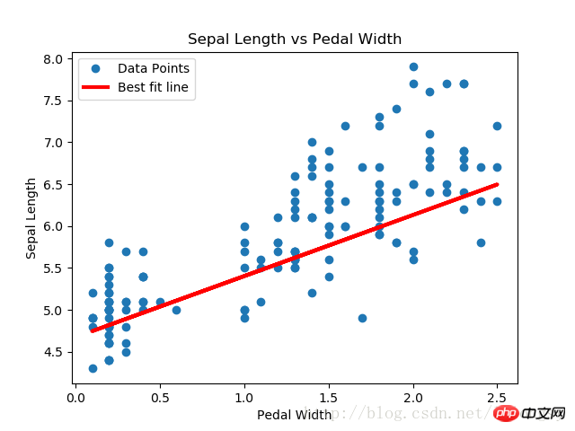
# Plot regression line against data points
plt.plot(x_vals, y_vals, 'o', label='Data Points')
plt.plot(x_vals, best_fit, 'r-', label='Best fit line', linewidth=3)
plt.legend(loc='upper left')
plt.title('Sepal Length vs Pedal Width')
plt.xlabel('Pedal Width')
plt.ylabel('Sepal Length')
plt.show()
# Plot loss over time
plt.plot(loss_vec, 'k-')
plt.title(regression_type + ' Loss per Generation')
plt.xlabel('Generation')
plt.ylabel('Loss')
plt.show()Output result:
Step #300 A = [[ 0.77170753]] b = [[ 1.82499862]]
Loss = [[ 10.26473045]]
Step #600 A = [[ 0.75908542]] b = [[ 3.2220633]]
Loss = [[ 3.06292033]]
Step #900 A = [[ 0.74843585] ] b = [[ 3.9975822]]
Loss = [[ 1.23220456]]
Step #1200 A = [[ 0.73752165]] b = [[ 4.42974091]]
Loss = [[ 0.57872057]]
Step #1500 A = [[ 0.72942668]] b = [[ 4.67253113]]
Loss = [[ 0.40874988]]
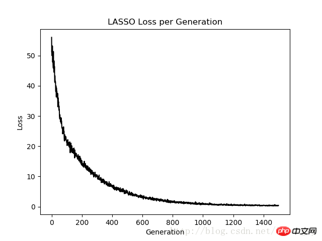
The lasso regression algorithm is implemented by adding a continuous step function based on the standard linear regression estimation. Due to the slope of the step function, we need to pay attention to the step size, as a step size that is too large will result in eventual non-convergence.
Related recommendations:
Example of using TensorFlow to implement Deming regression algorithm
The above is the detailed content of Examples of implementing lasso regression and ridge regression algorithms with TensorFlow. For more information, please follow other related articles on the PHP Chinese website!


![[Web front-end] Node.js quick start](https://img.php.cn/upload/course/000/000/067/662b5d34ba7c0227.png)


