
1. Number processing
1. Take absolute value =ABS(number)
2. Rounding=INT (number)
3. Rounding =ROUND (number, decimal places)
2. Judgment formula
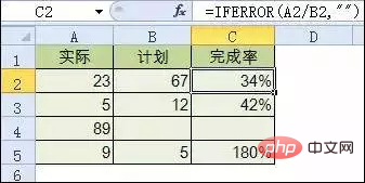
1. Errors caused by the formula The value is displayed as empty
Formula: C2=IFERROR(A2/B2,"")
Description: If it is an error value, it is displayed as empty, otherwise it is displayed normally.
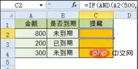
2. IF multi-condition judgment return value formula:
C2=IF(AND(A2
Explanation: Use AND if two conditions are true at the same time, or use the OR function if either condition is true.
3. Statistical formula
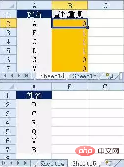
1. Statistics of repeated content in two tables
Formula: B2= COUNTIF(Sheet15!A:A,A2)
Note: If the return value is greater than 0, it means it exists in another table, and 0 means it does not exist.
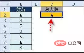
2. Count the total number of non-duplicate people
Formula: C2=SUMPRODUCT(1/COUNTIF(A2:A8,A2:A8))
Instructions: Use COUNTIF to count the number of occurrences of each person, use division by 1 to convert the number of occurrences into the denominator, and then add them up.
Related recommendations: "excel basic tutorial"
4. Summation formula
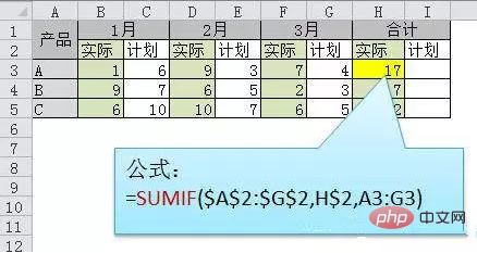
1. Sum every other column
Formula: H3=SUMIF($A$2:$G$2,H$2,A3:G3)
or=SUMPRODUCT((MOD(COLUMN( B3:G3),2)=0)*B3:G3)
Explanation: If there is no rule in the title row, use the second formula.
2. Single condition summation
Formula: F2=SUMIF(A:A,E2,C:C)
Explanation : Basic usage of SUMIF function.
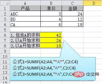
3. Single-condition fuzzy sum
Formula: See the figure below for details
Instructions: If you need to perform fuzzy sum, you need to master the use of wildcards, among which the asterisk It means any number of characters. For example, "*A*" means there are any number of characters before and after a, including A.
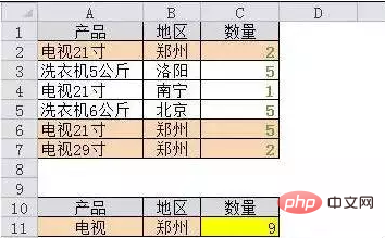
4. Multi-condition fuzzy summation
Formula: C11=SUMIFS(C2:C7,A2:A7,A11&"*",B2:B7 ,B11)
Note: You can use the wildcard character *
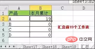
in sumifs. 5. Summing the same positions in multiple tables
Formula: b2 =SUM(Sheet1:Sheet19!B2)
Note: After deleting or adding a table in the middle of the table, the formula results will be automatically updated.
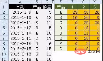
6. Sum by date and product
Formula: F2=SUMPRODUCT((MONTH($A$2:$A$25)=F$1) *($B$2: $B$25=$E2) *$C$2:$C$25)
Explanation: SUMPRODUCT can complete multi-condition summation.
5. Search and reference formulas
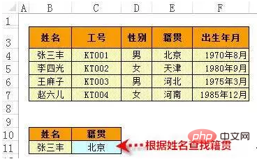
1. Single condition search formula
Formula 1: C11= VLOOKUP(B11,B3:F7,4,FALSE)
Description: Search is what VLOOKUP is best at, basic usage.
2. Bidirectional search formula
Formula=INDEX(C3:H7,MATCH(B10,B3:B7,0),MATCH(C10,C2 :H2,0))
Explanation: Use the MATCH function to find the position and the INDEX function to get the value.
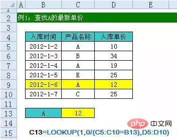
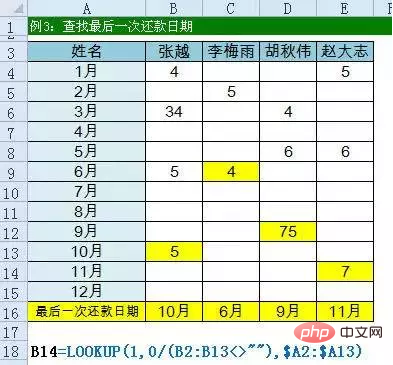
3. Find the last record that meets the conditions
Formula: See the figure below for details
Explanation: 0/(condition) can turn those that do not meet the conditions into error values , and lookup can ignore error values.
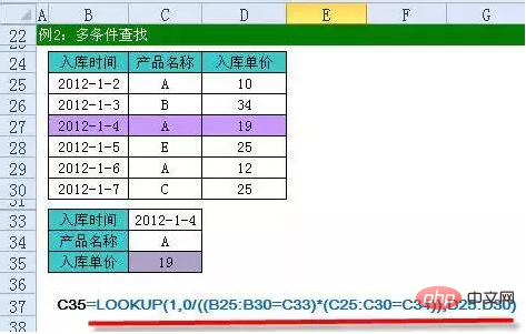
4. Multi-condition search
Formula: See the picture below for details
Explanation: The formula principle is the same as the previous formula
5. Find the last non-null value in the specified area
formula; see the figure below for details
Instructions: omitted
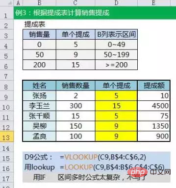
6. Get the corresponding value from the numerical range
Formula: See the figure below for details
Formula description: Both VLOOKUP and LOOKUP functions can be pressed When selecting interval values, it must be noted that the numbers in the sales column must be arranged in ascending order.
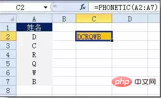
6. String processing formula
1. Multi-cell string merging
Formula: c2 =PHONETIC(A2:A7)
Explanation: The Phonetic function can only merge character content, not numbers.
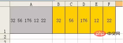
2. Cut off the part except the last 3 digits
Formula: =LEFT(D1,LEN(D1)-3)
Instructions: LEN calculates the total length, LEFT cuts the total length from the left to -3
3. Cut off the part before -
Formula: B2 =Left(A1,FIND("-",A1)-1)
Explanation: Use the FIND function to find the position and use LEFT to intercept.
4. Formula to intercept any segment of the string
Formula: B1=TRIM(MID(SUBSTITUTE($A1," ",REPT(" ",20)),20,20 ))
Explanation: The formula is intercepted by forcibly inserting N null characters.

5. String search
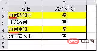
Formula: B2=IF(COUNT(FIND("Henan",A2))=0,"No", "Yes")
Explanation: FIND returns the position of the character if the search is successful, otherwise an error value is returned, and COUNT can count the number of numbers, which can be used to determine whether the search is successful.
6. String search one-to-many
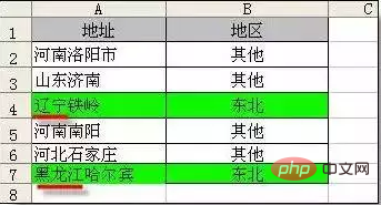
Formula: B2
=IF(COUNT(FIND({"Liaoning", "Heilongjiang","Jilin"},A2))=0,"Other","Northeast")
Instructions: Set the first parameter of FIND to a constant array, and use the COUNT function to count the FIND search results.
7. Date calculation formula
1. Calculation of the number of years, months and days between two dates
A1 is the start date (2011-12-1), and B1 is the end date (2013-6-10).
Calculation:
How many days apart? =datedif(A1,B1,"d") Result: 557
How many months apart? =datedif(A1,B1,"m") Result: 18
How many years apart? =datedif (A1,B1,"Y") Result: 1
Regardless of how many months are between years? =datedif(A1,B1,"Ym") Result: 6
How many days are there between years without considering it? =datedif(A1,B1,"YD") Result: 192
How many days are between the year and the month without considering it? =datedif(A1,B1,"MD") Result: 9
The third parameter description of the datedif function:
"Y" The number of whole years in the time period.
"M" The number of whole months in the time period.
"D" The number of days in the time period.
"MD" The difference in days. Ignore month and year in dates.
"YM" The difference in months. Ignore the day and year in the date.
"YD" The difference in days. Ignore the year in the date.
2. Number of working days after deducting weekend days
Formula: C2=NETWORKDAYS.INTL(IF(B2 Description: Returns all working days between two dates, use parameters to indicate which Which days are weekends and how many days are weekends. Weekends and any days designated as holidays are not considered working days. 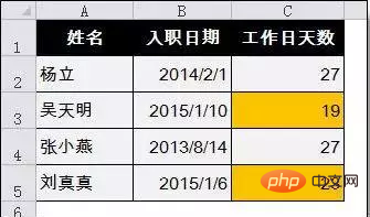
The above is the detailed content of Summary of all formulas of Excel functions. For more information, please follow other related articles on the PHP Chinese website!
 Compare the similarities and differences between two columns of data in excel
 excel duplicate item filter color
 How to copy an Excel table to make it the same size as the original
 Excel table slash divided into two
 Excel diagonal header is divided into two
 Absolute reference input method
 java export excel
 Excel input value is illegal


