很難說 Atlassian JIRA 是最受歡迎的問題追蹤器和專案管理解決方案之一。你可以喜歡它,也可以討厭它,但如果你被某家公司聘用為軟體工程師,那麼很有可能會遇到 JIRA。
如果您正在從事的專案非常活躍,可能會有數千個各種類型的 JIRA 問題。如果您領導工程師團隊,您可能會對分析工具感興趣,這些工具可以幫助您根據 JIRA 中儲存的資料來了解專案中發生的情況。 JIRA 整合了一些報告工具以及第三方插件。但其中大多數都是非常基本的。例如,很難找到相當靈活的「預測」工具。
專案越大,您對整合報告工具的滿意度就越低。在某些時候,您最終將使用 API 來提取、操作和視覺化資料。在過去 15 年的 JIRA 使用過程中,我看到了圍繞該領域的數十個採用各種程式語言的此類腳本和服務。
許多日常任務可能需要一次性資料分析,因此每次都編寫服務並沒有什麼回報。您可以將 JIRA 視為資料來源並使用典型的資料分析工具帶。例如,您可以使用 Jupyter,取得專案中最近的錯誤列表,準備「特徵」列表(對分析有價值的屬性),利用 pandas 計算統計數據,並嘗試使用 scikit-learn 預測趨勢。在這篇文章中,我想解釋一下如何做到這一點。
這裡我們要講的是雲版JIRA。但如果您使用的是自架版本,主要概念幾乎是相同的。
首先,我們需要建立一個金鑰來透過 REST API 存取 JIRA。為此,請前往設定檔管理- https://id.atlassian.com/manage-profile/profile-and-visibility 如果選擇「安全性」選項卡,您將找到「建立和管理API 令牌」連結:
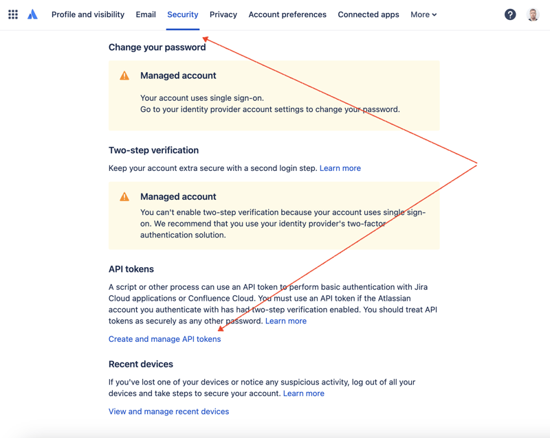
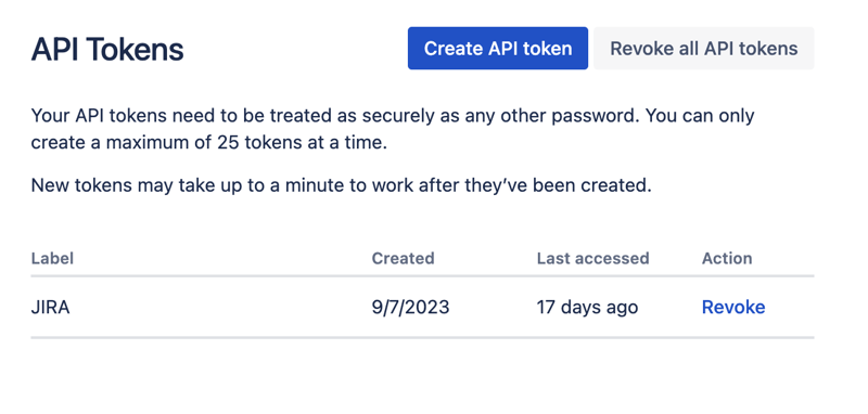
在此處建立一個新的 API 令牌並安全地儲存它。我們稍後會使用這個令牌。
處理資料集最方便的方法之一是使用 Jupyter。如果您不熟悉這個工具,請不要擔心。我將展示如何使用它來解決我們的問題。對於本地實驗,我喜歡使用 JetBrains 的 DataSpell,但也有免費的線上服務。 Kaggle 是資料科學家中最知名的服務之一。但是,他們的筆記本不允許您建立外部連接以透過 API 存取 JIRA。另一個非常受歡迎的服務是 Google 的 Colab。它允許您進行遠端連接並安裝額外的 Python 模組。
JIRA 有一個非常容易使用的 REST API。您可以使用您喜歡的 HTTP 請求方式進行 API 呼叫並手動解析回應。然而,我們將利用一個優秀且非常受歡迎的 jira 模組來實現此目的。
讓我們結合所有部分來找出解決方案。
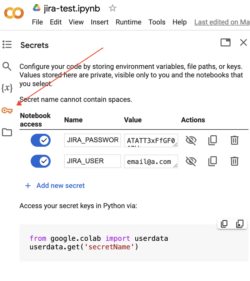
前往 Google Colab 介面並建立一個新筆記本。創建筆記本後,我們需要將先前獲得的 JIRA 憑證儲存為「秘密」。點擊左側工具列中的「金鑰」圖示以開啟對應的對話方塊並新增兩個具有以下名稱的「秘密」:JIRA_USER 和 JIRA_PASSWORD。在螢幕底部,您可以看到如何存取這些「秘密」:
接下來是安裝額外的 Python 模組以進行 JIRA 整合。我們可以透過在筆記本單元範圍內執行 shell 命令來做到這一點:
!pip install jira
輸出應如下圖所示:
Collecting jira
  Downloading jira-3.8.0-py3-none-any.whl (77 kB)
     ━━━━━━━━━━━━━━━━━━━━━━━━━━━━━━━━━━━━━━━━ 77.5/77.5 kB 1.3 MB/s eta 0:00:00
Requirement already satisfied: defusedxml in /usr/local/lib/python3.10/dist-packages (from jira) (0.7.1)
...
Installing collected packages: requests-toolbelt, jira
Successfully installed jira-3.8.0 requests-toolbelt-1.0.0
我們需要取得「秘密」/憑證:
from google.colab import userdata

JIRA_URL = 'https://******.atlassian.net'
JIRA_USER = userdata.get('JIRA_USER')
JIRA_PASSWORD = userdata.get('JIRA_PASSWORD')
並驗證與 JIRA Cloud 的連線:
from jira import JIRA

jira = JIRA(JIRA_URL, basic_auth=(JIRA_USER, JIRA_PASSWORD))
projects = jira.projects()
projects
如果連接正常且憑證有效,您應該會看到一個非空的項目清單:
[<JIRA Project: key='PROJ1', name='Name here..', id='10234'>,
 <JIRA Project: key='PROJ2', name='Friendly name..', id='10020'>,
 <JIRA Project: key='PROJ3', name='One more project', id='10045'>,
...
這樣我們就可以連接 JIRA 並從 JIRA 取得資料。下一步是獲取一些數據以使用 pandas 進行分析。讓我們試著取得某個項目在過去幾週內已解決問題的清單:
JIRA_FILTER = 19762

issues = jira.search_issues(
    f'filter={JIRA_FILTER}',
    maxResults=False,
    fields='summary,issuetype,assignee,reporter,aggregatetimespent',
)
我們需要將資料集轉換為 pandas 資料框:
import pandas as pd

df = pd.DataFrame([{
    'key': issue.key,
    'assignee': issue.fields.assignee and issue.fields.assignee.displayName or issue.fields.reporter.displayName,
    'time': issue.fields.aggregatetimespent,
    'summary': issue.fields.summary,
} for issue in issues])

df.set_index('key', inplace=True)

df
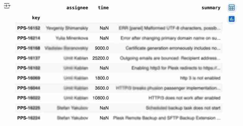
輸出可能如下圖所示:
We would like to analyze how much time it usually takes to solve the issue. People are not ideal, so sometimes they forget to log the work. It brings a headache if you try to analyze such data using JIRA built-in tools. But it's not a problem for us to make some adjustments using pandas. For example, we can transform the "time" field from seconds into hours and replace the absent values with the median value (beware, dropna can be more suitable if there are a lot of gaps):
df['time'].fillna(df['time'].median(), inplace=True)
df['time'] = df['time'] / 3600
We can easily visualize the distribution to find out anomalies:
df['time'].plot.bar(xlabel='', xticks=[])
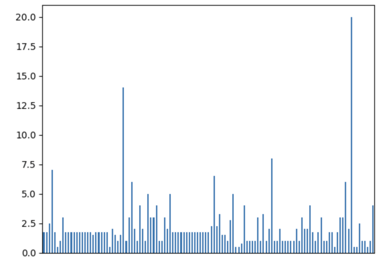
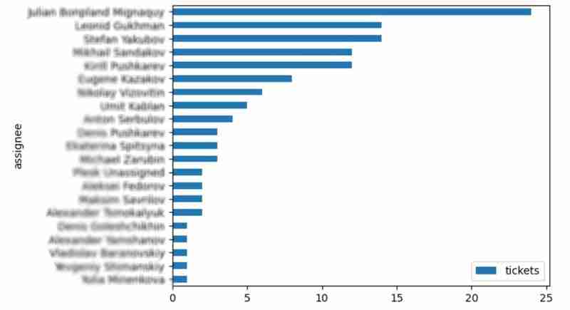
It is also interesting to see the distribution of solved problems by the assignee:
top_solvers = df.groupby('assignee').count()[['time']]
top_solvers.rename(columns={'time': 'tickets'}, inplace=True)
top_solvers.sort_values('tickets', ascending=False, inplace=True)

top_solvers.plot.barh().invert_yaxis()
It may look like the following:
Let's try to predict the amount of time required to finish all open issues. Of course, we can do it without machine learning by using simple approximation and the average time to resolve the issue. So the predicted amount of required time is the number of open issues multiplied by the average time to resolve one. For example, the median time to solve one issue is 2 hours, and we have 9 open issues, so the time required to solve them all is 18 hours (approximation). It's a good enough forecast, but we might know the speed of solving depends on the product, team, and other attributes of the issue. If we want to improve the prediction, we can utilize machine learning to solve this task.
The high-level approach looks the following:
For the first step, we will use a dataset of tickets for the last 30 weeks. Some parts here are simplified for illustrative purposes. In real life, the amount of data for learning should be big enough to make a useful model (e.g., in our case, we need thousands of issues to be analyzed).
issues = jira.search_issues(
    f'project = PPS AND status IN (Resolved) AND created >= -30w',
    maxResults=False,
    fields='summary,issuetype,customfield_10718,customfield_10674,aggregatetimespent',
)

closed_tickets = pd.DataFrame([{
    'key': issue.key,
    'team': issue.fields.customfield_10718,
    'product': issue.fields.customfield_10674,
    'time': issue.fields.aggregatetimespent,
} for issue in issues])

closed_tickets.set_index('key', inplace=True)
closed_tickets['time'].fillna(closed_tickets['time'].median(), inplace=True)

closed_tickets
In my case, it's something around 800 tickets and only two fields for "learning": "team" and "product."
The next step is to obtain our target dataset. Why do I do it so early? I want to clean up and do "feature engineering" in one shot for both datasets. Otherwise, the mismatch between the structures can cause problems.
issues = jira.search_issues(
    f'project = PPS AND status IN (Open, Reopened)',
    maxResults=False,
    fields='summary,issuetype,customfield_10718,customfield_10674',
)

open_tickets = pd.DataFrame([{
    'key': issue.key,
    'team': issue.fields.customfield_10718,
    'product': issue.fields.customfield_10674,
} for issue in issues])

open_tickets.set_index('key', inplace=True)

open_tickets
Please notice we have no "time" column here because we want to predict it. Let's nullify it and combine both datasets to prepare the "features."
open_tickets['time'] = 0
tickets = pd.concat([closed_tickets, open_tickets])

tickets
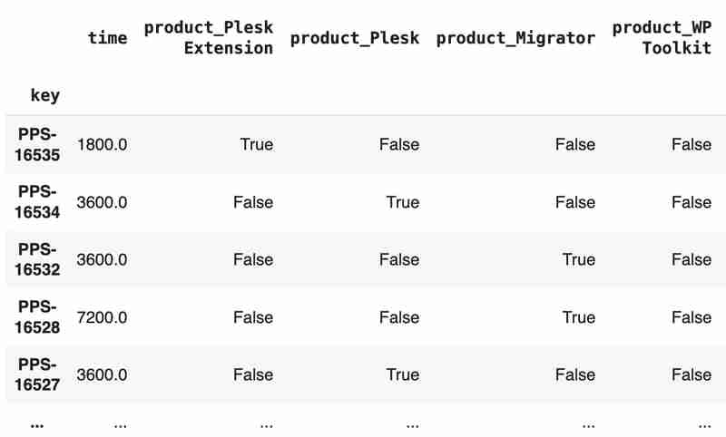
Columns "team" and "product" contain string values. One of the ways of dealing with that is to transform each value into separate fields with boolean flags.
products = pd.get_dummies(tickets['product'], prefix='product')
tickets = pd.concat([tickets, products], axis=1)
tickets.drop('product', axis=1, inplace=True)

teams = pd.get_dummies(tickets['team'], prefix='team')
tickets = pd.concat([tickets, teams], axis=1)
tickets.drop('team', axis=1, inplace=True)

tickets
The result may look like the following:
After the combined dataset preparation, we can split it back into two parts:
closed_tickets = tickets[:len(closed_tickets)]
open_tickets = tickets[len(closed_tickets):][:]
Now it's time to train our model:
from sklearn.model_selection import train_test_split
from sklearn.tree import DecisionTreeRegressor

features = closed_tickets.drop(['time'], axis=1)
labels = closed_tickets['time']

features_train, features_val, labels_train, labels_val = train_test_split(features, labels, test_size=0.2)

model = DecisionTreeRegressor()
model.fit(features_train, labels_train)
model.score(features_val, labels_val)
And the final step is to use our model to make a prediction:
open_tickets['time'] = model.predict(open_tickets.drop('time', axis=1, errors='ignore'))
open_tickets['time'].sum() / 3600
The final output, in my case, is 25 hours, which is higher than our initial rough estimation. This was a basic example. However, by using ML tools, you can significantly expand your abilities to analyze JIRA data.
Sometimes, JIRA built-in tools and plugins are not sufficient for effective analysis. Moreover, many 3rd party plugins are rather expensive, costing thousands of dollars per year, and you will still struggle to make them work the way you want. However, you can easily utilize well-known data analysis tools by fetching necessary information via JIRA API and go beyond these limitations. I spent so many hours playing with various JIRA plugins in attempts to create good reports for projects, but they often missed some important parts. Building a tool or a full-featured service on top of JIRA API also often looks like overkill. That's why typical data analysis and ML tools like Jupiter, pandas, matplotlib, scikit-learn, and others may work better here.

以上是使用 Pandas 進行 JIRA 分析的詳細內容。更多資訊請關注PHP中文網其他相關文章!


