

#excel中的價值錯誤:原因和修復

Whether it's a simple formatting mistake or a more complex syntax issue, knowing how to fix #VALUE errors in Excel is essential for anyone who wants to create error-free spreadsheets and ensure the accuracy of their data.
When working with Excel, it is common to encounter errors. One of the most frustrating errors is #VALUE, which is raised when a formula or function is unable to process data. This error can be caused by several factors including incorrect syntax, mismatched cell references, or hidden characters. In this article, we will explore the various causes of the #VALUE error and provide tips on how to fix it.
When is #VALUE error raised in Excel?
The #VALUE! error in Excel is commonly caused by the following reasons:
- Unexpected data type. If an Excel function requires a specific data type, such as a number or text, and a cell contains a different data type.
- Incorrect formula syntax. When the function's arguments are incorrect, missing or in wrong order.
- Spaces. If a formula refers to a cell that contains a space character. Visually, such cells look absolutely empty.
- Invisible characters. Sometimes, cells may contain hidden or non-printing characters that prevent a formula from calculating correctly.
- Dates formatted as text. When dates are input in the format that Excel does not understand, they are treated as text strings rather than valid dates.
- Ranges have incompatible dimensions. When formula references a few ranges that are not of the same size or shape, Excel cannot calculate the formula and throws an error.
As you see, the #VALUE error in Excel can be caused by a variety of factors. By understanding the root cause, you can more easily find the right remedy to fix it.

How to troubleshoot and fix #VALUE error in Excel
Once you identify the cause of the error, use the appropriate troubleshooting steps to resolve the issue.
Check if data type is valid
To avoid the #VALUE error in Excel, verify that the data type in the referred cell is correct. If a formula or function requires numeric data, make sure the cell contains a number and not text.
A typical example is math operations such as addition and multiplication. When one of the values that you add up or multiply is non-numeric, a #VALUE error occurs:

To fix the error, you can use one of these options:
- Enter the missing numeric values.
- Use Excel functions that automatically ignore text values.
- Write an IF statement that corresponds to your business logic.
In this example, you can use the PRODUCT function:
=PRODUCT(B3, C3)
If one of the referenced cells contains text, logical value, or is empty, that cell is ignored. The result is as if you multiply the other value by 1.
Alternatively, you can build an IF statement like this:
=IF(AND(ISNUMBER(B3), ISNUMBER(C3)), B3*C3, 0)
This formula multiplies two cells only if both values are numeric and returns zero if either cell contains a non-numeric value. For this particular case, it makes perfect sense.

Remove spaces and hidden characters
In some formulas, a cell with errant spaces or invisible characters may also cause a #VALUE! error, as shown in the screenshot below:

Visually, cells such as D3, B7 and C14 may appear to be completely empty. However, they do contain one or more spaces or non-printing characters. In Excel, a space character is considered text, and it can potentially trigger the #VALUE! error. In fact, it is just another case of the previous example, so it can be fixed in a similar manner:
- Ensure that the problematic cells are really empty. To do this, select the cell and press the Delete key to remove any hidden character in it.
- Use an Excel function that ignores text values, such as the SUM function instead of the arithmetic operation of addition.

Verify that referred ranges are compatible
Many Excel functions that accept multiple ranges in their arguments require those ranges to be of the same size and shape. If not, a formula raises the #VALUE error.
For example, the dynamic array FILTER function results in a #VALUE error when the include and array arguments have incompatible dimensions. For example:
=FILTER(A3:B20, A3:A22="Apple")
Once the range references are changed accordingly, the error is gone:
=FILTER(A3:B20, A3:A20="Apple")

Make sure dates are not stored as text
In Excel, dates are typically stored as numeric values. However, some dates in your worksheet may be stored as text strings instead. When this happens, Excel will return the #VALUE! error if you try to perform calculations or operations on these dates, as text values cannot be added, subtracted or somehow else calculated.
To resolve this issue, you need to convert text-formatted dates to valid Excel dates.

Check formula syntax
Another possible cause of a #VALUE error in Excel could be a syntax error in your formula. Excel's Formula Auditing tools can help you identify and correct such issues.
- Select the cell with the formula that is producing the #VALUE error.
- On the Formulas tab, in the Formula Auditing group, click on Evaluate Formula or Error Checking.
Excel will step through the formula one section at a time, showing the result of each step. If there is a syntax error, Excel will highlight the specific part of the formula is causing the error. Once you have detected the syntax error, correct it and re-evaluate the formula to ensure that it is now working as expected.
For example, consider the following formula in the dataset below:
=SORT(CHOOSECOLS(A3:B20, 3))
The #VALUE error occurs because the col_num argument (3) of the CHOOSECOLS function is greater than the total number of columns in the referred array (2).

Setting the last argument to 2 resolves the issue and returns the desired result – the Total column sorted from smallest to largest:

#VALUE error in Excel XLOOKUP and VLOOKUP
The VLOOKUP function and its modern successor XLOOKUP are commonly used in Excel to search and retrieve matching data. However, both functions can produce the #VALUE error under certain circumstances.
One common cause of the #VALUE error in XLOOKUP is when the dimensions of the lookup and return arrays are incomparable. For example, you cannot search in a horizontal array and return values from a vertical array. Also, the lookup array cannot be bigger or smaller than the return array. If there is any mismatch in the size of these arrays, XLOOKUP will not be able to perform the lookup and return the #VALUE error.
For example, the below XLOOKUP formula returns a #VALUE error because the lookup and return arrays contain a different number of rows:
=XLOOKUP(D3, A3:A20, B3:B22)
Adjusting the return_array reference resolves the error:
=XLOOKUP(D3, A3:A20, B3:B20)

In VLOOKUP, two common reasons for the #VALUE error are when the lookup value exceeds 255 characters and when the col_index_num argument is less than 1. For more information, please see #VALUE error in VLOOKUP.
Get rid of #VALUE error using IFERROR function
To eliminate the #VALUE error in your Excel sheets, you can use the IFERROR function in Excel 2007 - 365 or the IF ISERROR combination in earlier versions.
Suppose you are using a DATEDIF formula to find the difference between the dates in B3 and C3:
=DATEDIF(B3, C3, "d")
If one or both dates are invalid, the formula results in a #VALUE error. To fix it, wrap your core formula in the IFERROR function like this:
=IFERROR(DATEDIF(B3, C3, "d"), "Invalid date!")
If Excel doesn't recognize the referenced cell value as a date, the IFERROR function will explicitly point it out.

Tip. To quickly find all #VALUE errors in a worksheet, you can utilize the Go to Special feature or the Find and Replace dialog box. We discussed these options in detail when locating #NAME errors. For #VALUE errors, the steps are essentially the same.
That's how to detect and fix the #VALUE error in Excel. By understanding the causes and using the appropriate troubleshooting techniques, you can quickly get your spreadsheet back on track.
Practice workbook for download
#VALUE error in Excel - examples (.xlsx file)
以上是#excel中的價值錯誤:原因和修復的詳細內容。更多資訊請關注PHP中文網其他相關文章!

熱AI工具

Undresser.AI Undress
人工智慧驅動的應用程序,用於創建逼真的裸體照片

AI Clothes Remover
用於從照片中去除衣服的線上人工智慧工具。

Undress AI Tool
免費脫衣圖片

Clothoff.io
AI脫衣器

Video Face Swap
使用我們完全免費的人工智慧換臉工具,輕鬆在任何影片中換臉!

熱門文章
熱工具

記事本++7.3.1
好用且免費的程式碼編輯器

SublimeText3漢化版
中文版,非常好用

禪工作室 13.0.1
強大的PHP整合開發環境

Dreamweaver CS6
視覺化網頁開發工具

SublimeText3 Mac版
神級程式碼編輯軟體(SublimeText3)


 如何使用示例使用Flash Fill ofecl
Apr 05, 2025 am 09:15 AM
如何使用示例使用Flash Fill ofecl
Apr 05, 2025 am 09:15 AM
本教程為Excel的Flash Fill功能提供了綜合指南,這是一種可自動化數據輸入任務的強大工具。 它涵蓋了從定義和位置到高級用法和故障排除的各個方面。 了解Excel的FLA

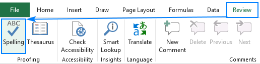 如何在Excel中拼寫檢查
Apr 06, 2025 am 09:10 AM
如何在Excel中拼寫檢查
Apr 06, 2025 am 09:10 AM
該教程展示了在Excel中進行拼寫檢查的各種方法:手動檢查,VBA宏和使用專用工具。 學習檢查單元格,範圍,工作表和整個工作簿中的拼寫。 雖然Excel不是文字處理器,但它的spel
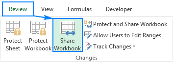 Excel共享工作簿:如何為多個用戶共享Excel文件
Apr 11, 2025 am 11:58 AM
Excel共享工作簿:如何為多個用戶共享Excel文件
Apr 11, 2025 am 11:58 AM
本教程提供了共享Excel工作簿,涵蓋各種方法,訪問控制和衝突解決方案的綜合指南。 現代Excel版本(2010年,2013年,2016年及以後)簡化了協作編輯,消除了M的需求
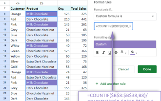 Google電子表格Countif函數帶有公式示例
Apr 11, 2025 pm 12:03 PM
Google電子表格Countif函數帶有公式示例
Apr 11, 2025 pm 12:03 PM
Google主張Countif:綜合指南 本指南探討了Google表中的多功能Countif函數,展示了其超出簡單單元格計數的應用程序。 我們將介紹從精確和部分比賽到Han的各種情況
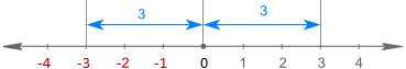 Excel中的絕對值:ABS功能與公式示例
Apr 06, 2025 am 09:12 AM
Excel中的絕對值:ABS功能與公式示例
Apr 06, 2025 am 09:12 AM
本教程解釋了絕對價值的概念,並演示了ABS函數的實用Excel應用,以計算數據集中的絕對值。 數字可能是正面的或負數的,但有時只有正值是需要的
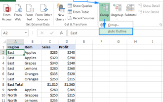 Excel:組行自動或手動,崩潰並擴展行
Apr 08, 2025 am 11:17 AM
Excel:組行自動或手動,崩潰並擴展行
Apr 08, 2025 am 11:17 AM
本教程演示瞭如何通過對行進行分組來簡化複雜的Excel電子表格,從而使數據易於分析。學會快速隱藏或顯示行組,並將整個輪廓崩潰到特定的級別。 大型的詳細電子表格可以是
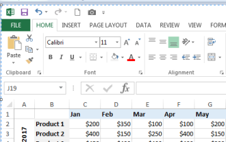 如何將Excel轉換為JPG-保存.xls或.xlsx作為圖像文件
Apr 11, 2025 am 11:31 AM
如何將Excel轉換為JPG-保存.xls或.xlsx作為圖像文件
Apr 11, 2025 am 11:31 AM
本教程探討了將.xls文件轉換為.jpg映像的各種方法,包括內置的Windows工具和免費的在線轉換器。 需要創建演示文稿,安全共享電子表格數據或設計文檔嗎?轉換喲
