
import osimport pandas as pdfrom PIL import Imagedef crop_cell(row):"""crop_cell(row)given a pd.Series row of the dataframe, load row['filename'] with PIL,crop it to the box row['xmin'], row['xmax'], row['ymin'], row['ymax']save the cropped image,return cropped filename"""input_dir = 'BCCDJPEGImages'output_dir = 'BCCDcropped'# open imageim = Image.open(f"{input_dir}{row['filename']}")# size of the image in pixelswidth, height = im.size# setting the points for cropped imageleft = row['xmin']bottom = row['ymax']right = row['xmax']top = row['ymin']# cropped imageim1 = im.crop((left, top, right, bottom))cropped_fname = f"BloodImage_{row['image_id']:03d}_{row['cell_id']:02d}.jpg"# shows the image in image viewer# im1.show()# save imagetry:im1.save(f"{output_dir}{cropped_fname}")except:return 'error while saving image'return cropped_fnameif __name__ == "__main__":# load labels csv into Pandas DataFramefilepath = "BCCDdataset2-masterlabels.csv"df = pd.read_csv(filepath)# iterate through cells, crop each cell, and save cropped cell to filedataset_df['cell_filename'] = dataset_df.apply(crop_cell, axis=1)
淺析細胞影像資料的主動學習

透過細胞影像的標籤對模型表現的影響,為資料設定優先權和權重。
許多機器學習任務的主要障礙之一是缺乏標記資料。而標記資料可能會耗費很長的時間,而且很昂貴,因此很多時候嘗試使用機器學習方法來解決問題是不合理的。
為了解決這個問題,機器學習領域出現了一個叫做主動學習的領域。主動學習是機器學習中的一種方法,它提供了一個框架,根據模型已經看到的標記資料對未標記的資料樣本進行優先排序。如果想
細胞成像的分割和分類等技術是一個快速發展的領域研究。就像在其他機器學習領域一樣,數據的標註是非常昂貴的,而且對於數據標註的品質要求也非常的高。針對這個問題,本篇文章介紹一種對紅血球和白血球影像分類任務的主動學習端到端工作流程。
我們的目標是將生物學和主動學習的結合,並幫助其他人使用主動學習方法解決生物學領域中類似的和更複雜的任務。
本篇文章主要由三個部分組成:
- 細胞影像預處理-這裡將介紹如何預處理未分割的血球影像。
- 使用CellProfiler提取細胞特徵-展示如何從生物細胞照片影像中提取形態學特徵,以用作機器學習模型的特徵。
- 使用主動學習-展示一個模擬使用主動學習和不使用主動學習的對比實驗。
細胞影像預處理
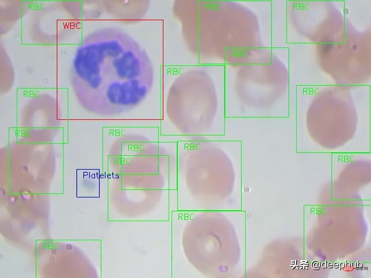
我們將使用在MIT許可的血球影像資料集(GitHub和Kaggle)。每張圖片都根據紅血球(RBC)和白血球(WBC)分類進行標記。對於這4種白血球(嗜酸性球、淋巴球、單核球和嗜中性球)還有附加的標籤,但在本文的研究中並沒有使用這些標籤。
下面是一個來自資料集的全尺寸原始影像的範例:
#建立樣本DF
原始資料集包含一個export .py腳本,它將XML註解解析為一個CSV表,其中包含每個細胞的檔案名稱、細胞類型標籤和邊界框。
原始腳本沒有包含cell_id列,但我們要對單一細胞進行分類,所以我們稍微修改了程式碼,新增了該列並新增了一列包括image_id和cell_id的filename列:
import os, sys, randomimport xml.etree.ElementTree as ETfrom glob import globimport pandas as pdfrom shutil import copyfileannotations = glob('BCCD_Dataset/BCCD/Annotations/*.xml')df = []for file in annotations:#filename = file.split('/')[-1].split('.')[0] + '.jpg'#filename = str(cnt) + '.jpg'filename = file.split('\')[-1]filename =filename.split('.')[0] + '.jpg'row = []parsedXML = ET.parse(file)cell_id = 0for node in parsedXML.getroot().iter('object'):blood_cells = node.find('name').textxmin = int(node.find('bndbox/xmin').text)xmax = int(node.find('bndbox/xmax').text)ymin = int(node.find('bndbox/ymin').text)ymax = int(node.find('bndbox/ymax').text)row = [filename, cell_id, blood_cells, xmin, xmax, ymin, ymax]df.append(row)cell_id += 1data = pd.DataFrame(df, columns=['filename', 'cell_id', 'cell_type', 'xmin', 'xmax', 'ymin', 'ymax'])data['image_id'] = data['filename'].apply(lambda x: int(x[-7:-4]))data[['filename', 'image_id', 'cell_id', 'cell_type', 'xmin', 'xmax', 'ymin', 'ymax']].to_csv('bccd.csv', index=False)裁剪
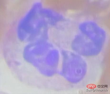
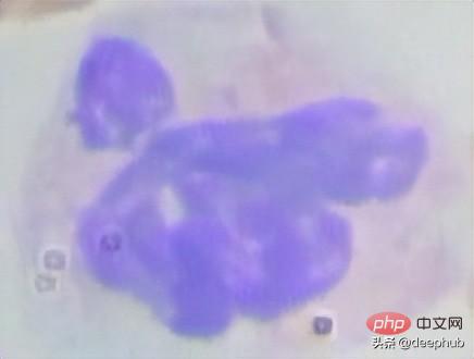
為了能夠處理數據,第一步是根據邊界框座標裁剪全尺寸圖像。這就產生了很多大小不一的細胞圖像:


import osimport pandas as pdfrom PIL import Imagedef crop_cell(row):"""crop_cell(row)given a pd.Series row of the dataframe, load row['filename'] with PIL,crop it to the box row['xmin'], row['xmax'], row['ymin'], row['ymax']save the cropped image,return cropped filename"""input_dir = 'BCCDJPEGImages'output_dir = 'BCCDcropped'# open imageim = Image.open(f"{input_dir}{row['filename']}")# size of the image in pixelswidth, height = im.size# setting the points for cropped imageleft = row['xmin']bottom = row['ymax']right = row['xmax']top = row['ymin']# cropped imageim1 = im.crop((left, top, right, bottom))cropped_fname = f"BloodImage_{row['image_id']:03d}_{row['cell_id']:02d}.jpg"# shows the image in image viewer# im1.show()# save imagetry:im1.save(f"{output_dir}{cropped_fname}")except:return 'error while saving image'return cropped_fnameif __name__ == "__main__":# load labels csv into Pandas DataFramefilepath = "BCCDdataset2-masterlabels.csv"df = pd.read_csv(filepath)# iterate through cells, crop each cell, and save cropped cell to filedataset_df['cell_filename'] = dataset_df.apply(crop_cell, axis=1)登入後複製
以上就是我們所做的所有預處理操作。現在,我們繼續使用CellProfiler來擷取特徵。 使用CellProfiler提取細胞特徵CellProfiler是一個免費的開源影像分析軟體,可以從大規模細胞影像中自動定量測量。 CellProfiler還包含一個GUI介面,允許我們可視化的操作先下載CellProfiler,如果CellProfiler無法打開,則可能需要安裝Visual C 發布包,具體安裝方式參考官網。 開啟軟體就可以載入映像了, 如果想要建立管道可以在CellProfiler官網找到其提供的可用的功能清單。大多數功能分為三個主要群組:影像處理,目標的處理和測量。 常用的功能如下:import osimport pandas as pdfrom PIL import Imagedef crop_cell(row):"""crop_cell(row)given a pd.Series row of the dataframe, load row['filename'] with PIL,crop it to the box row['xmin'], row['xmax'], row['ymin'], row['ymax']save the cropped image,return cropped filename"""input_dir = 'BCCDJPEGImages'output_dir = 'BCCDcropped'# open imageim = Image.open(f"{input_dir}{row['filename']}")# size of the image in pixelswidth, height = im.size# setting the points for cropped imageleft = row['xmin']bottom = row['ymax']right = row['xmax']top = row['ymin']# cropped imageim1 = im.crop((left, top, right, bottom))cropped_fname = f"BloodImage_{row['image_id']:03d}_{row['cell_id']:02d}.jpg"# shows the image in image viewer# im1.show()# save imagetry:im1.save(f"{output_dir}{cropped_fname}")except:return 'error while saving image'return cropped_fnameif __name__ == "__main__":# load labels csv into Pandas DataFramefilepath = "BCCDdataset2-masterlabels.csv"df = pd.read_csv(filepath)# iterate through cells, crop each cell, and save cropped cell to filedataset_df['cell_filename'] = dataset_df.apply(crop_cell, axis=1)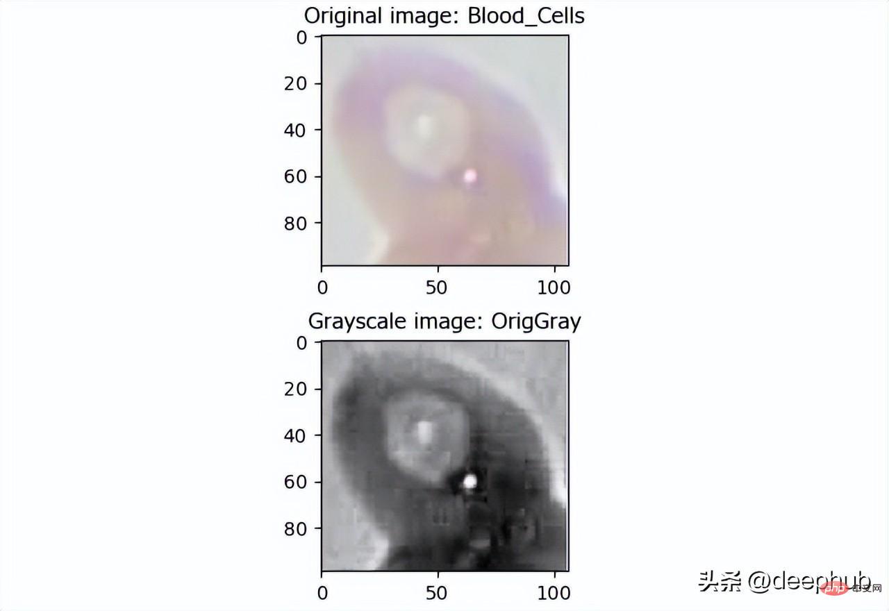 影像處理- 轉為灰階圖:
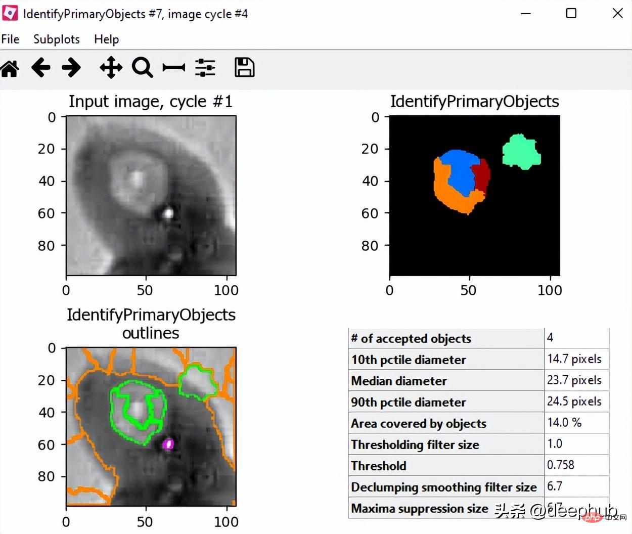
测量 - 测量对象强度
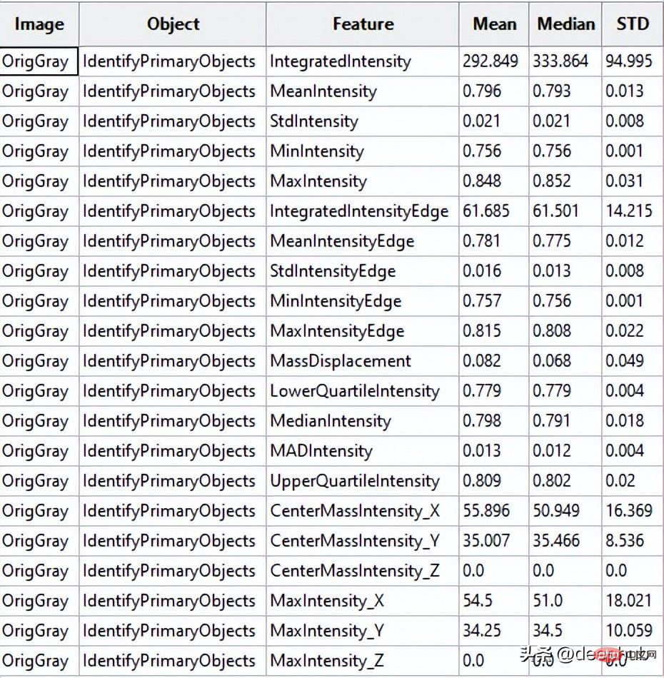
CellProfiler可以将输出为CSV文件或者保存指定数据库中。这里我们将输出保存为CSV文件,然后将其加载到Python进行进一步处理。
说明:CellProfiler还可以将你处理图像的流程保存并进行分享。
主动学习
我们现在已经有了训练需要的搜有数据,现在可以开始试验使用主动学习策略是否可以通过更少的数据标记获得更高的准确性。 我们的假设是:使用主动学习可以通过大量减少在细胞分类任务上训练机器学习模型所需的标记数据量来节省宝贵的时间和精力。
主动学习框架
在深入研究实验之前,我们希望对modAL进行快速介绍: modAL是Python的活跃学习框架。 它提供了Sklearn API,因此可以非常容易的将其集成到代码中。 该框架可以轻松地使用不同的主动学习策略。 他们的文档也很清晰,所以建议从它开始你的一个主动学习项目。
主动学习与随机学习
为了验证假设,我们将进行一项实验,将添加新标签数据的随机子抽样策略与主动学习策略进行比较。开始用一些相同的标记样本训练2个Logistic回归估计器。然后将在一个模型中使用随机策略,在第二个模型中使用主动学习策略。
我们首先为实验准备数据,加载由Cell Profiler言创建的特征。 这里过滤了无色血细胞的血小板,只保留红和白细胞(将问题简化,并减少数据量) 。所以现在我们正在尝试解决二进制分类问题 - RBC与WBC。使用Sklearn Label的label encoder进行编码,并拆分数据集进行训练和测试。
# imports for the whole experimentimport numpy as npfrom matplotlib import pyplot as pltfrom modAL import ActiveLearnerimport pandas as pdfrom modAL.uncertainty import uncertainty_samplingfrom sklearn import preprocessingfrom sklearn.metrics import , average_precision_scorefrom sklearn.linear_model import LogisticRegression# upload the cell profiler features for each celldata = pd.read_csv('Zaretski_Image_All.csv')# filter plateletsdata = data[data['cell_type'] != 'Platelets']# define the labeltarget = 'cell_type'label_encoder = preprocessing.LabelEncoder()y = label_encoder.fit_transform(data[target])# take the learning features onlyX = data.iloc[:, 5:]# create training and testing setsX_train, X_test, y_train, y_test = train_test_split(X.to_numpy(), y, test_size=0.33, random_state=42)下一步就是创建模型
<span style="color: rgb(89, 89, 89); margin: 0px; padding: 0px; background: none 0% 0% / auto repeat scroll padding-box border-box rgba(0, 0, 0, 0);">dummy_learner</span> <span style="color: rgb(215, 58, 73); margin: 0px; padding: 0px; background: none 0% 0% / auto repeat scroll padding-box border-box rgba(0, 0, 0, 0);">=</span> <span style="color: rgb(89, 89, 89); margin: 0px; padding: 0px; background: none 0% 0% / auto repeat scroll padding-box border-box rgba(0, 0, 0, 0);">LogisticRegression</span>()<br><span style="color: rgb(89, 89, 89); margin: 0px; padding: 0px; background: none 0% 0% / auto repeat scroll padding-box border-box rgba(0, 0, 0, 0);">active_learner</span> <span style="color: rgb(215, 58, 73); margin: 0px; padding: 0px; background: none 0% 0% / auto repeat scroll padding-box border-box rgba(0, 0, 0, 0);">=</span> <span style="color: rgb(89, 89, 89); margin: 0px; padding: 0px; background: none 0% 0% / auto repeat scroll padding-box border-box rgba(0, 0, 0, 0);">ActiveLearner</span>(<br><span style="color: rgb(89, 89, 89); margin: 0px; padding: 0px; background: none 0% 0% / auto repeat scroll padding-box border-box rgba(0, 0, 0, 0);">estimator</span><span style="color: rgb(215, 58, 73); margin: 0px; padding: 0px; background: none 0% 0% / auto repeat scroll padding-box border-box rgba(0, 0, 0, 0);">=</span><span style="color: rgb(89, 89, 89); margin: 0px; padding: 0px; background: none 0% 0% / auto repeat scroll padding-box border-box rgba(0, 0, 0, 0);">LogisticRegression</span>(),<br><span style="color: rgb(89, 89, 89); margin: 0px; padding: 0px; background: none 0% 0% / auto repeat scroll padding-box border-box rgba(0, 0, 0, 0);">query_strategy</span><span style="color: rgb(215, 58, 73); margin: 0px; padding: 0px; background: none 0% 0% / auto repeat scroll padding-box border-box rgba(0, 0, 0, 0);">=</span><span style="color: rgb(89, 89, 89); margin: 0px; padding: 0px; background: none 0% 0% / auto repeat scroll padding-box border-box rgba(0, 0, 0, 0);">uncertainty_sampling</span>()<br>)
dummy_learner是使用随机策略的模型,而active_learner是使用主动学习策略的模型。为了实例化一个主动学习模型,我们使用modAL包中的ActiveLearner对象。在“estimator”字段中,可以插入任何sklearnAPI兼容的模型。在query_strategy '字段中可以选择特定的主动学习策略。这里使用“uncertainty_sampling()”。这方面更多的信息请查看modAL文档。
将训练数据分成两组。第一个是训练数据,我们知道它的标签,会用它来训练模型。第二个是验证数据,虽然标签也是已知的,但是我们假装不知道它的标签,并通过模型预测的标签和实际标签进行比较来评估模型的性能。然后我们将训练的数据样本数设置成5。
# the training size that we will start withbase_size = 5# the 'base' data that will be the training set for our modelX_train_base_dummy = X_train[:base_size]X_train_base_active = X_train[:base_size]y_train_base_dummy = y_train[:base_size]y_train_base_active = y_train[:base_size]# the 'new' data that will simulate unlabeled data that we pick a sample from and label itX_train_new_dummy = X_train[base_size:]X_train_new_active = X_train[base_size:]y_train_new_dummy = y_train[base_size:]y_train_new_active = y_train[base_size:]
我们训练298个epoch,在每个epoch中,将训练这俩个模型和选择下一个样本,并根据每个模型的策略选择是否将样本加入到我们的“基础”数据中,并在每个epoch中测试其准确性。因为分类是不平衡的,所以使用平均精度评分来衡量模型的性能。
在随机策略中选择下一个样本,只需将下一个样本添加到虚拟数据集的“新”组中,这是因为数据集已经是打乱的的,因此不需要在进行这个操作。对于主动学习,将使用名为“query”的ActiveLearner方法,该方法获取“新”组的未标记数据,并返回他建议添加到训练“基础”组的样本索引。被选择的样本都将从组中删除,因此样本只能被选择一次。
# arrays to accumulate the scores of each simulation along the epochsdummy_scores = []active_scores = []# number of desired epochsrange_epoch = 298# running the experimentfor i in range(range_epoch):# train the models on the 'base' datasetactive_learner.fit(X_train_base_active, y_train_base_active)dummy_learner.fit(X_train_base_dummy, y_train_base_dummy)# evaluate the modelsdummy_pred = dummy_learner.predict(X_test)active_pred = active_learner.predict(X_test)# accumulate the scoresdummy_scores.append(average_precision_score(dummy_pred, y_test))active_scores.append(average_precision_score(active_pred, y_test))# pick the next sample in the random strategy and randomly# add it to the 'base' dataset of the dummy learner and remove it from the 'new' datasetX_train_base_dummy = np.append(X_train_base_dummy, [X_train_new_dummy[0, :]], axis=0)y_train_base_dummy = np.concatenate([y_train_base_dummy, np.array([y_train_new_dummy[0]])], axis=0)X_train_new_dummy = X_train_new_dummy[1:]y_train_new_dummy = y_train_new_dummy[1:]# pick next sample in the active strategyquery_idx, query_sample = active_learner.query(X_train_new_active)# add the index to the 'base' dataset of the active learner and remove it from the 'new' datasetX_train_base_active = np.append(X_train_base_active, X_train_new_active[query_idx], axis=0)y_train_base_active = np.concatenate([y_train_base_active, y_train_new_active[query_idx]], axis=0)X_train_new_active = np.concatenate([X_train_new_active[:query_idx[0]], X_train_new_active[query_idx[0] + 1:]], axis=0)y_train_new_active = np.concatenate([y_train_new_active[:query_idx[0]], y_train_new_active[query_idx[0] + 1:]], axis=0)
结果如下:
plt.plot(list(range(range_epoch)), active_scores, label='Active Learning')plt.plot(list(range(range_epoch)), dummy_scores, label='Dummy')plt.xlabel('number of added samples')plt.ylabel('average precision score')plt.legend(loc='lower right')plt.savefig("models robustness vs dummy.png", bbox_inches='tight')plt.show()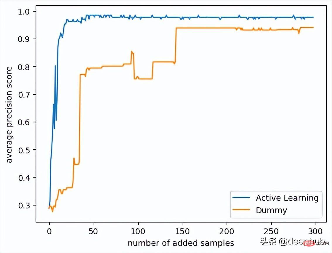
策略之间的差异还是很大的,可以看到主动学习只使用25个样本就可以达到平均精度0.9得分! 而使用随机的策略则需要175个样本才能达到相同的精度!
此外主動學習策略的模型的分數接近0.99,而隨機模型的分數在0.95左右停止了!如果我們使用所有數據,那麼它們最終分數是相同的,但是我們的研究目的是在少量標註數據的前提下訓練,所以只使用了數據集中的300個隨機樣本。
總結
本文展示了將主動學習用於細胞成像任務的好處。主動學習是機器學習中的一組方法,可根據其標籤對模型效能的影響來優先考慮未標記的資料範例的解決方案。由於標記資料是一項涉及許多資源(金錢和時間)的任務,因此判斷那些標記那些樣本可以最大程度地提高模型的表現是非常必要的。
細胞成像為生物學,醫學和藥理學領域做出了巨大貢獻。先前分析細胞影像需要有價值的專業人力資本,但是像主動學習這種技術的出現為醫學領域這種需要大量人力標註資料集的領域提供了一個非常好的解決方案。
以上是淺析細胞影像資料的主動學習的詳細內容。更多資訊請關注PHP中文網其他相關文章!

熱AI工具

Undresser.AI Undress
人工智慧驅動的應用程序,用於創建逼真的裸體照片

AI Clothes Remover
用於從照片中去除衣服的線上人工智慧工具。

Undress AI Tool
免費脫衣圖片

Clothoff.io
AI脫衣器

Video Face Swap
使用我們完全免費的人工智慧換臉工具,輕鬆在任何影片中換臉!

熱門文章
熱工具

記事本++7.3.1
好用且免費的程式碼編輯器

SublimeText3漢化版
中文版,非常好用

禪工作室 13.0.1
強大的PHP整合開發環境

Dreamweaver CS6
視覺化網頁開發工具

SublimeText3 Mac版
神級程式碼編輯軟體(SublimeText3)


 15個值得推薦的開源免費圖片標註工具
Mar 28, 2024 pm 01:21 PM
15個值得推薦的開源免費圖片標註工具
Mar 28, 2024 pm 01:21 PM
圖像標註是將標籤或描述性資訊與圖像相關聯的過程,以賦予圖像內容更深層的含義和解釋。這個過程對於機器學習至關重要,它有助於訓練視覺模型以更準確地識別圖像中的各個元素。透過為圖像添加標註,使得電腦能夠理解圖像背後的語義和上下文,從而提高對圖像內容的理解和分析能力。影像標註的應用範圍廣泛,涵蓋了許多領域,如電腦視覺、自然語言處理和圖視覺模型具有廣泛的應用領域,例如,輔助車輛識別道路上的障礙物,幫助疾病的檢測和診斷透過醫學影像識別。本文主要推薦一些較好的開源免費的圖片標註工具。 1.Makesens
 一文帶您了解SHAP:機器學習的模型解釋
Jun 01, 2024 am 10:58 AM
一文帶您了解SHAP:機器學習的模型解釋
Jun 01, 2024 am 10:58 AM
在機器學習和資料科學領域,模型的可解釋性一直是研究者和實踐者關注的焦點。隨著深度學習和整合方法等複雜模型的廣泛應用,理解模型的決策過程變得尤為重要。可解釋人工智慧(ExplainableAI|XAI)透過提高模型的透明度,幫助建立對機器學習模型的信任和信心。提高模型的透明度可以透過多種複雜模型的廣泛應用等方法來實現,以及用於解釋模型的決策過程。這些方法包括特徵重要性分析、模型預測區間估計、局部可解釋性演算法等。特徵重要性分析可以透過評估模型對輸入特徵的影響程度來解釋模型的決策過程。模型預測區間估計
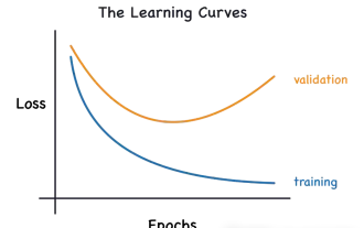 透過學習曲線辨識過擬合和欠擬合
Apr 29, 2024 pm 06:50 PM
透過學習曲線辨識過擬合和欠擬合
Apr 29, 2024 pm 06:50 PM
本文將介紹如何透過學習曲線來有效辨識機器學習模型中的過度擬合和欠擬合。欠擬合和過擬合1、過擬合如果一個模型對資料進行了過度訓練,以至於它從中學習了噪聲,那麼這個模型就被稱為過擬合。過度擬合模型非常完美地學習了每一個例子,所以它會錯誤地分類一個看不見的/新的例子。對於一個過度擬合的模型,我們會得到一個完美/接近完美的訓練集分數和一個糟糕的驗證集/測試分數。略有修改:"過擬合的原因:用一個複雜的模型來解決一個簡單的問題,從資料中提取雜訊。因為小資料集作為訓練集可能無法代表所有資料的正確表示。"2、欠擬合如
 人工智慧在太空探索和人居工程中的演變
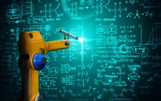
Apr 29, 2024 pm 03:25 PM
人工智慧在太空探索和人居工程中的演變
Apr 29, 2024 pm 03:25 PM
1950年代,人工智慧(AI)誕生。當時研究人員發現機器可以執行類似人類的任務,例如思考。後來,在1960年代,美國國防部資助了人工智慧,並建立了實驗室進行進一步開發。研究人員發現人工智慧在許多領域都有用武之地,例如太空探索和極端環境中的生存。太空探索是對宇宙的研究,宇宙涵蓋了地球以外的整個宇宙空間。太空被歸類為極端環境,因為它的條件與地球不同。要在太空中生存,必須考慮許多因素,並採取預防措施。科學家和研究人員認為,探索太空並了解一切事物的現狀有助於理解宇宙的運作方式,並為潛在的環境危機
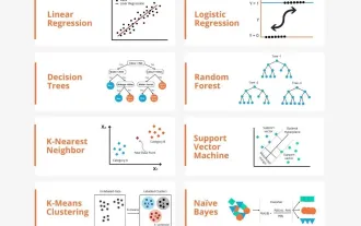 通透!機器學習各大模型原理的深度剖析!
Apr 12, 2024 pm 05:55 PM
通透!機器學習各大模型原理的深度剖析!
Apr 12, 2024 pm 05:55 PM
通俗來說,機器學習模型是一種數學函數,它能夠將輸入資料映射到預測輸出。更具體地說,機器學習模型是一種透過學習訓練數據,來調整模型參數,以最小化預測輸出與真實標籤之間的誤差的數學函數。在機器學習中存在多種模型,例如邏輯迴歸模型、決策樹模型、支援向量機模型等,每種模型都有其適用的資料類型和問題類型。同時,不同模型之間存在著許多共通性,或者說有一條隱藏的模型演化的路徑。將聯結主義的感知機為例,透過增加感知機的隱藏層數量,我們可以將其轉化為深度神經網路。而對感知機加入核函數的話就可以轉換為SVM。這一
 使用C++實現機器學習演算法:常見挑戰及解決方案
Jun 03, 2024 pm 01:25 PM
使用C++實現機器學習演算法:常見挑戰及解決方案
Jun 03, 2024 pm 01:25 PM
C++中機器學習演算法面臨的常見挑戰包括記憶體管理、多執行緒、效能最佳化和可維護性。解決方案包括使用智慧指標、現代線程庫、SIMD指令和第三方庫,並遵循程式碼風格指南和使用自動化工具。實作案例展示如何利用Eigen函式庫實現線性迴歸演算法,有效地管理記憶體和使用高效能矩陣操作。
 你所不知道的機器學習五大學派
Jun 05, 2024 pm 08:51 PM
你所不知道的機器學習五大學派
Jun 05, 2024 pm 08:51 PM
機器學習是人工智慧的重要分支,它賦予電腦從數據中學習的能力,並能夠在無需明確編程的情況下改進自身能力。機器學習在各個領域都有廣泛的應用,從影像辨識和自然語言處理到推薦系統和詐欺偵測,它正在改變我們的生活方式。機器學習領域存在著多種不同的方法和理論,其中最具影響力的五種方法被稱為「機器學習五大派」。這五大派分別為符號派、聯結派、進化派、貝葉斯派和類推學派。 1.符號學派符號學(Symbolism),又稱符號主義,強調利用符號進行邏輯推理和表達知識。該學派認為學習是一種逆向演繹的過程,透過現有的
 Flash Attention穩定嗎? Meta、哈佛發現其模型權重偏差呈現數量級波動
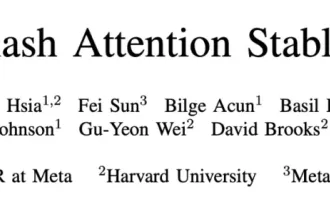
May 30, 2024 pm 01:24 PM
Flash Attention穩定嗎? Meta、哈佛發現其模型權重偏差呈現數量級波動
May 30, 2024 pm 01:24 PM
MetaFAIR聯合哈佛優化大規模機器學習時所產生的資料偏差,提供了新的研究架構。據所周知,大語言模型的訓練常常需要數月的時間,使用數百甚至上千個GPU。以LLaMA270B模型為例,其訓練總共需要1,720,320個GPU小時。由於這些工作負載的規模和複雜性,導致訓練大模型存在著獨特的系統性挑戰。最近,許多機構在訓練SOTA生成式AI模型時報告了訓練過程中的不穩定情況,它們通常以損失尖峰的形式出現,例如Google的PaLM模型訓練過程中出現了多達20次的損失尖峰。數值偏差是造成這種訓練不準確性的根因,
