很难说 Atlassian JIRA 是最受欢迎的问题跟踪器和项目管理解决方案之一。你可以喜欢它,也可以讨厌它,但如果你被某家公司聘用为软件工程师,那么很有可能会遇到 JIRA。
如果您正在从事的项目非常活跃,可能会有数千个各种类型的 JIRA 问题。如果您领导着一个工程师团队,您可能会对分析工具感兴趣,这些工具可以帮助您根据 JIRA 中存储的数据了解项目中发生的情况。 JIRA 集成了一些报告工具以及第三方插件。但其中大多数都是非常基本的。例如,很难找到相当灵活的“预测”工具。
项目越大,您对集成报告工具的满意度就越低。在某些时候,您最终将使用 API 来提取、操作和可视化数据。在过去 15 年的 JIRA 使用过程中,我看到了围绕该领域的数十个采用各种编程语言的此类脚本和服务。
许多日常任务可能需要一次性数据分析,因此每次都编写服务并没有什么回报。您可以将 JIRA 视为数据源并使用典型的数据分析工具带。例如,您可以使用 Jupyter,获取项目中最近的错误列表,准备“特征”列表(对分析有价值的属性),利用 pandas 计算统计数据,并尝试使用 scikit-learn 预测趋势。在这篇文章中,我想解释一下如何做到这一点。
这里我们要讲的是云版JIRA。但如果您使用的是自托管版本,主要概念几乎是相同的。
首先,我们需要创建一个密钥来通过 REST API 访问 JIRA。为此,请转到配置文件管理 - https://id.atlassian.com/manage-profile/profile-and-visibility 如果选择“安全”选项卡,您将找到“创建和管理 API 令牌”链接:
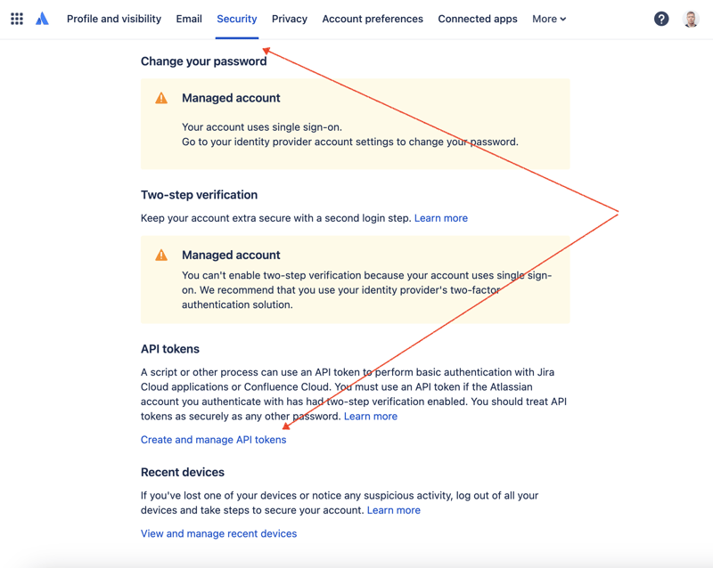
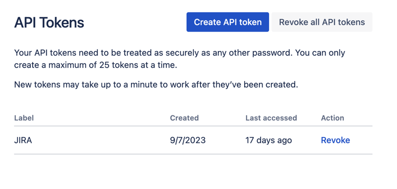
在此处创建一个新的 API 令牌并安全地存储它。我们稍后会使用这个令牌。
处理数据集最方便的方法之一是使用 Jupyter。如果您不熟悉这个工具,请不要担心。我将展示如何使用它来解决我们的问题。对于本地实验,我喜欢使用 JetBrains 的 DataSpell,但也有免费的在线服务。 Kaggle 是数据科学家中最知名的服务之一。但是,他们的笔记本不允许您建立外部连接以通过 API 访问 JIRA。另一项非常受欢迎的服务是 Google 的 Colab。它允许您进行远程连接并安装额外的 Python 模块。
JIRA 有一个非常易于使用的 REST API。您可以使用您最喜欢的 HTTP 请求方式进行 API 调用并手动解析响应。然而,我们将利用一个优秀且非常流行的 jira 模块来实现此目的。
让我们结合所有部分来找出解决方案。
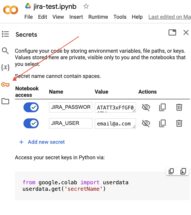
转到 Google Colab 界面并创建一个新笔记本。创建笔记本后,我们需要将之前获得的 JIRA 凭据存储为“秘密”。单击左侧工具栏中的“密钥”图标打开相应的对话框并添加两个具有以下名称的“秘密”:JIRA_USER 和 JIRA_PASSWORD。在屏幕底部,您可以看到如何访问这些“秘密”:
接下来是安装额外的 Python 模块以进行 JIRA 集成。我们可以通过在笔记本单元范围内执行 shell 命令来做到这一点:
!pip install jira
输出应如下所示:
Collecting jira
  Downloading jira-3.8.0-py3-none-any.whl (77 kB)
     ━━━━━━━━━━━━━━━━━━━━━━━━━━━━━━━━━━━━━━━━ 77.5/77.5 kB 1.3 MB/s eta 0:00:00
Requirement already satisfied: defusedxml in /usr/local/lib/python3.10/dist-packages (from jira) (0.7.1)
...
Installing collected packages: requests-toolbelt, jira
Successfully installed jira-3.8.0 requests-toolbelt-1.0.0
我们需要获取“秘密”/凭证:
from google.colab import userdata

JIRA_URL = 'https://******.atlassian.net'
JIRA_USER = userdata.get('JIRA_USER')
JIRA_PASSWORD = userdata.get('JIRA_PASSWORD')
并验证与 JIRA Cloud 的连接:
from jira import JIRA

jira = JIRA(JIRA_URL, basic_auth=(JIRA_USER, JIRA_PASSWORD))
projects = jira.projects()
projects
如果连接正常并且凭据有效,您应该会看到一个非空的项目列表:
[<JIRA Project: key='PROJ1', name='Name here..', id='10234'>,
 <JIRA Project: key='PROJ2', name='Friendly name..', id='10020'>,
 <JIRA Project: key='PROJ3', name='One more project', id='10045'>,
...
这样我们就可以连接 JIRA 并从 JIRA 获取数据了。下一步是获取一些数据以使用 pandas 进行分析。让我们尝试获取某个项目在过去几周内已解决问题的列表:
JIRA_FILTER = 19762

issues = jira.search_issues(
    f'filter={JIRA_FILTER}',
    maxResults=False,
    fields='summary,issuetype,assignee,reporter,aggregatetimespent',
)
我们需要将数据集转换为 pandas 数据框:
import pandas as pd

df = pd.DataFrame([{
    'key': issue.key,
    'assignee': issue.fields.assignee and issue.fields.assignee.displayName or issue.fields.reporter.displayName,
    'time': issue.fields.aggregatetimespent,
    'summary': issue.fields.summary,
} for issue in issues])

df.set_index('key', inplace=True)

df
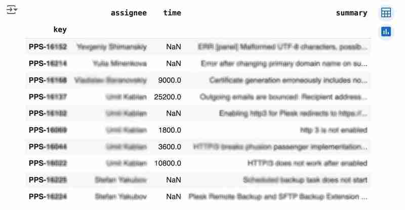
输出可能如下所示:
We would like to analyze how much time it usually takes to solve the issue. People are not ideal, so sometimes they forget to log the work. It brings a headache if you try to analyze such data using JIRA built-in tools. But it's not a problem for us to make some adjustments using pandas. For example, we can transform the "time" field from seconds into hours and replace the absent values with the median value (beware, dropna can be more suitable if there are a lot of gaps):
df['time'].fillna(df['time'].median(), inplace=True)
df['time'] = df['time'] / 3600
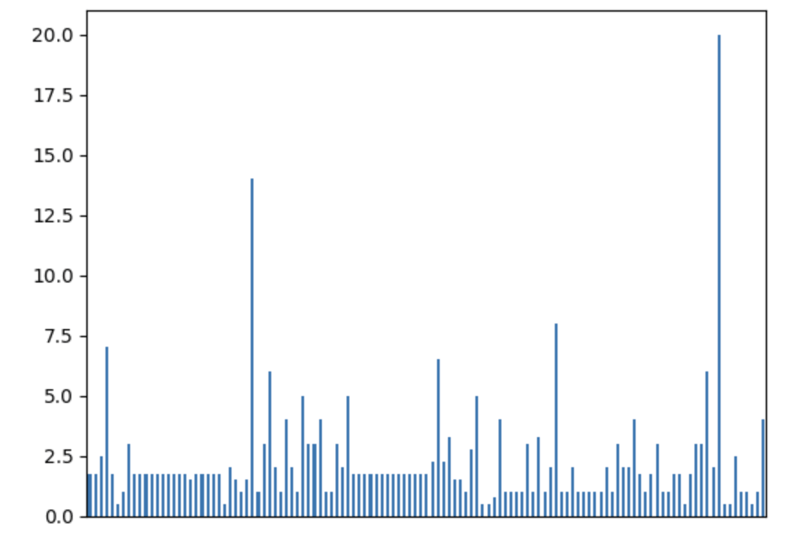
We can easily visualize the distribution to find out anomalies:
df['time'].plot.bar(xlabel='', xticks=[])
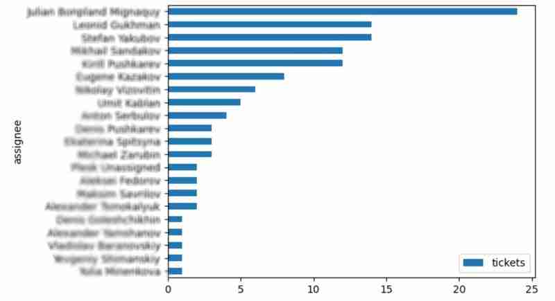
It is also interesting to see the distribution of solved problems by the assignee:
top_solvers = df.groupby('assignee').count()[['time']]
top_solvers.rename(columns={'time': 'tickets'}, inplace=True)
top_solvers.sort_values('tickets', ascending=False, inplace=True)

top_solvers.plot.barh().invert_yaxis()
It may look like the following:
Let's try to predict the amount of time required to finish all open issues. Of course, we can do it without machine learning by using simple approximation and the average time to resolve the issue. So the predicted amount of required time is the number of open issues multiplied by the average time to resolve one. For example, the median time to solve one issue is 2 hours, and we have 9 open issues, so the time required to solve them all is 18 hours (approximation). It's a good enough forecast, but we might know the speed of solving depends on the product, team, and other attributes of the issue. If we want to improve the prediction, we can utilize machine learning to solve this task.
The high-level approach looks the following:
For the first step, we will use a dataset of tickets for the last 30 weeks. Some parts here are simplified for illustrative purposes. In real life, the amount of data for learning should be big enough to make a useful model (e.g., in our case, we need thousands of issues to be analyzed).
issues = jira.search_issues(
    f'project = PPS AND status IN (Resolved) AND created >= -30w',
    maxResults=False,
    fields='summary,issuetype,customfield_10718,customfield_10674,aggregatetimespent',
)

closed_tickets = pd.DataFrame([{
    'key': issue.key,
    'team': issue.fields.customfield_10718,
    'product': issue.fields.customfield_10674,
    'time': issue.fields.aggregatetimespent,
} for issue in issues])

closed_tickets.set_index('key', inplace=True)
closed_tickets['time'].fillna(closed_tickets['time'].median(), inplace=True)

closed_tickets
In my case, it's something around 800 tickets and only two fields for "learning": "team" and "product."
The next step is to obtain our target dataset. Why do I do it so early? I want to clean up and do "feature engineering" in one shot for both datasets. Otherwise, the mismatch between the structures can cause problems.
issues = jira.search_issues(
    f'project = PPS AND status IN (Open, Reopened)',
    maxResults=False,
    fields='summary,issuetype,customfield_10718,customfield_10674',
)

open_tickets = pd.DataFrame([{
    'key': issue.key,
    'team': issue.fields.customfield_10718,
    'product': issue.fields.customfield_10674,
} for issue in issues])

open_tickets.set_index('key', inplace=True)

open_tickets
Please notice we have no "time" column here because we want to predict it. Let's nullify it and combine both datasets to prepare the "features."
open_tickets['time'] = 0
tickets = pd.concat([closed_tickets, open_tickets])

tickets
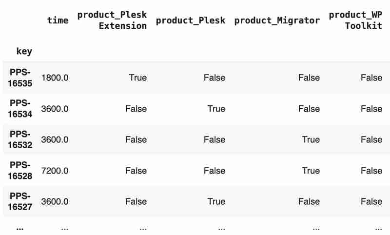
Columns "team" and "product" contain string values. One of the ways of dealing with that is to transform each value into separate fields with boolean flags.
products = pd.get_dummies(tickets['product'], prefix='product')
tickets = pd.concat([tickets, products], axis=1)
tickets.drop('product', axis=1, inplace=True)

teams = pd.get_dummies(tickets['team'], prefix='team')
tickets = pd.concat([tickets, teams], axis=1)
tickets.drop('team', axis=1, inplace=True)

tickets
The result may look like the following:
After the combined dataset preparation, we can split it back into two parts:
closed_tickets = tickets[:len(closed_tickets)]
open_tickets = tickets[len(closed_tickets):][:]
Now it's time to train our model:
from sklearn.model_selection import train_test_split
from sklearn.tree import DecisionTreeRegressor

features = closed_tickets.drop(['time'], axis=1)
labels = closed_tickets['time']

features_train, features_val, labels_train, labels_val = train_test_split(features, labels, test_size=0.2)

model = DecisionTreeRegressor()
model.fit(features_train, labels_train)
model.score(features_val, labels_val)
And the final step is to use our model to make a prediction:
open_tickets['time'] = model.predict(open_tickets.drop('time', axis=1, errors='ignore'))
open_tickets['time'].sum() / 3600
The final output, in my case, is 25 hours, which is higher than our initial rough estimation. This was a basic example. However, by using ML tools, you can significantly expand your abilities to analyze JIRA data.
Sometimes, JIRA built-in tools and plugins are not sufficient for effective analysis. Moreover, many 3rd party plugins are rather expensive, costing thousands of dollars per year, and you will still struggle to make them work the way you want. However, you can easily utilize well-known data analysis tools by fetching necessary information via JIRA API and go beyond these limitations. I spent so many hours playing with various JIRA plugins in attempts to create good reports for projects, but they often missed some important parts. Building a tool or a full-featured service on top of JIRA API also often looks like overkill. That's why typical data analysis and ML tools like Jupiter, pandas, matplotlib, scikit-learn, and others may work better here.

以上是使用 Pandas 进行 JIRA 分析的详细内容。更多信息请关注PHP中文网其他相关文章!


