python绘制三维图的详细教程

本篇文章给大家带来了关于Python的相关知识，通常我们用 Python 绘制的都是二维平面图,但有时也需要绘制三维场景图,下面介绍了关于python绘制三维图的相关资料，希望对大家有帮助。

【相关推荐：Python3视频教程 】

本文仅仅梳理最基本的绘图方法。

一、初始化

假设已经安装了matplotlib工具包。

利用matplotlib.figure.Figure创建一个图框：

import matplotlib.pyplot as plt
from mpl_toolkits.mplot3d import Axes3D
fig = plt.figure()
ax = fig.add_subplot(111, projection='3d')

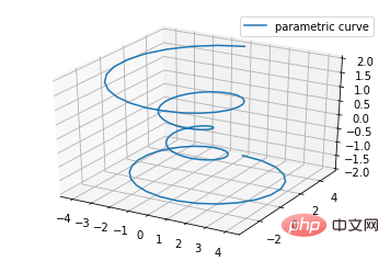
二、直线绘制（Line plots）

基本用法：

ax.plot(x,y,z,label=' ')

code:

import matplotlib as mpl
from mpl_toolkits.mplot3d import Axes3D
import numpy as np
import matplotlib.pyplot as plt
 
mpl.rcParams['legend.fontsize'] = 10
 
fig = plt.figure()
ax = fig.gca(projection='3d')
theta = np.linspace(-4 * np.pi, 4 * np.pi, 100)
z = np.linspace(-2, 2, 100)
r = z**2 + 1
x = r * np.sin(theta)
y = r * np.cos(theta)
ax.plot(x, y, z, label='parametric curve')
ax.legend()
 
plt.show()

三、散点绘制（Scatter plots）

基本用法：

ax.scatter(xs, ys, zs, s=20, c=None, depthshade=True, *args, *kwargs)

• xs,ys,zs：输入数据；
• s:scatter点的尺寸
• c:颜色，如c = 'r'就是红色；
• depthshase:透明化，True为透明，默认为True，False为不透明
• *args等为扩展变量，如maker = 'o'，则scatter结果为’o‘的形状

code:

from mpl_toolkits.mplot3d import Axes3D
import matplotlib.pyplot as plt
import numpy as np
 
 
def randrange(n, vmin, vmax):
    '''
    Helper function to make an array of random numbers having shape (n, )
    with each number distributed Uniform(vmin, vmax).
    '''
    return (vmax - vmin)*np.random.rand(n) + vmin
 
fig = plt.figure()
ax = fig.add_subplot(111, projection='3d')
 
n = 100
 
# For each set of style and range settings, plot n random points in the box
# defined by x in [23, 32], y in [0, 100], z in [zlow, zhigh].
for c, m, zlow, zhigh in [('r', 'o', -50, -25), ('b', '^', -30, -5)]:
    xs = randrange(n, 23, 32)
    ys = randrange(n, 0, 100)
    zs = randrange(n, zlow, zhigh)
    ax.scatter(xs, ys, zs, c=c, marker=m)
 
ax.set_xlabel('X Label')
ax.set_ylabel('Y Label')
ax.set_zlabel('Z Label')
 
plt.show()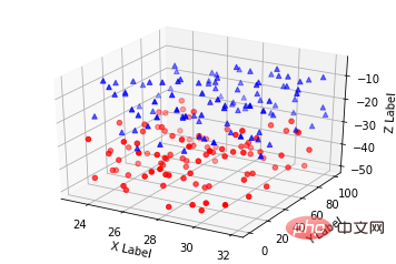

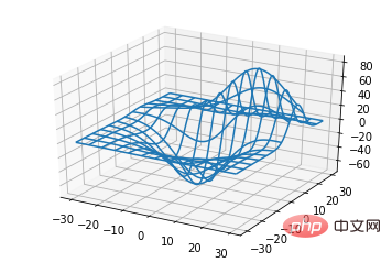
四、线框图（Wireframe plots）

基本用法：

ax.plot_wireframe(X, Y, Z, *args, **kwargs)

• X,Y,Z：输入数据
• rstride:行步长
• cstride:列步长
• rcount:行数上限
• ccount:列数上限

code:

from mpl_toolkits.mplot3d import axes3d
import matplotlib.pyplot as plt
 
 
fig = plt.figure()
ax = fig.add_subplot(111, projection='3d')
 
# Grab some test data.
X, Y, Z = axes3d.get_test_data(0.05)
 
# Plot a basic wireframe.
ax.plot_wireframe(X, Y, Z, rstride=10, cstride=10)
 
plt.show()

五、表面图（Surface plots）

基本用法：

ax.plot_surface(X, Y, Z, *args, **kwargs)

• X,Y,Z：数据
• rstride、cstride、rcount、ccount:同Wireframe plots定义
• color:表面颜色
• cmap:图层

code:

from mpl_toolkits.mplot3d import Axes3D
import matplotlib.pyplot as plt
from matplotlib import cm
from matplotlib.ticker import LinearLocator, FormatStrFormatter
import numpy as np
 
 
fig = plt.figure()
ax = fig.gca(projection='3d')
 
# Make data.
X = np.arange(-5, 5, 0.25)
Y = np.arange(-5, 5, 0.25)
X, Y = np.meshgrid(X, Y)
R = np.sqrt(X**2 + Y**2)
Z = np.sin(R)
 
# Plot the surface.
surf = ax.plot_surface(X, Y, Z, cmap=cm.coolwarm,
                       linewidth=0, antialiased=False)
 
# Customize the z axis.
ax.set_zlim(-1.01, 1.01)
ax.zaxis.set_major_locator(LinearLocator(10))
ax.zaxis.set_major_formatter(FormatStrFormatter('%.02f'))
 
# Add a color bar which maps values to colors.
fig.colorbar(surf, shrink=0.5, aspect=5)
 
plt.show()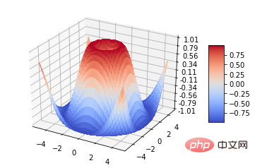

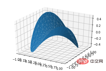
六、三角表面图（Tri-Surface plots）

基本用法：

ax.plot_trisurf(*args, **kwargs)

• X,Y,Z:数据
• 其他参数类似surface-plot

code:

from mpl_toolkits.mplot3d import Axes3D
import matplotlib.pyplot as plt
import numpy as np
 
 
n_radii = 8
n_angles = 36
 
# Make radii and angles spaces (radius r=0 omitted to eliminate duplication).
radii = np.linspace(0.125, 1.0, n_radii)
angles = np.linspace(0, 2*np.pi, n_angles, endpoint=False)
 
# Repeat all angles for each radius.
angles = np.repeat(angles[..., np.newaxis], n_radii, axis=1)
 
# Convert polar (radii, angles) coords to cartesian (x, y) coords.
# (0, 0) is manually added at this stage,  so there will be no duplicate
# points in the (x, y) plane.
x = np.append(0, (radii*np.cos(angles)).flatten())
y = np.append(0, (radii*np.sin(angles)).flatten())
 
# Compute z to make the pringle surface.
z = np.sin(-x*y)
 
fig = plt.figure()
ax = fig.gca(projection='3d')
 
ax.plot_trisurf(x, y, z, linewidth=0.2, antialiased=True)
 
plt.show()

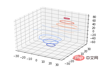
七、等高线（Contour plots）

基本用法：

ax.contour(X, Y, Z, *args, **kwargs)

code:

from mpl_toolkits.mplot3d import axes3d
import matplotlib.pyplot as plt
from matplotlib import cm
 
fig = plt.figure()
ax = fig.add_subplot(111, projection='3d')
X, Y, Z = axes3d.get_test_data(0.05)
cset = ax.contour(X, Y, Z, cmap=cm.coolwarm)
ax.clabel(cset, fontsize=9, inline=1)
 
plt.show()

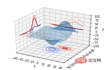
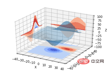
二维的等高线，同样可以配合三维表面图一起绘制：

code:

from mpl_toolkits.mplot3d import axes3d
from mpl_toolkits.mplot3d import axes3d
import matplotlib.pyplot as plt
from matplotlib import cm
 
fig = plt.figure()
ax = fig.gca(projection='3d')
X, Y, Z = axes3d.get_test_data(0.05)
ax.plot_surface(X, Y, Z, rstride=8, cstride=8, alpha=0.3)
cset = ax.contour(X, Y, Z, zdir='z', offset=-100, cmap=cm.coolwarm)
cset = ax.contour(X, Y, Z, zdir='x', offset=-40, cmap=cm.coolwarm)
cset = ax.contour(X, Y, Z, zdir='y', offset=40, cmap=cm.coolwarm)
 
ax.set_xlabel('X')
ax.set_xlim(-40, 40)
ax.set_ylabel('Y')
ax.set_ylim(-40, 40)
ax.set_zlabel('Z')
ax.set_zlim(-100, 100)
 
plt.show()

也可以是三维等高线在二维平面的投影：

code:

from mpl_toolkits.mplot3d import axes3d
import matplotlib.pyplot as plt
from matplotlib import cm
 
fig = plt.figure()
ax = fig.gca(projection='3d')
X, Y, Z = axes3d.get_test_data(0.05)
ax.plot_surface(X, Y, Z, rstride=8, cstride=8, alpha=0.3)
cset = ax.contourf(X, Y, Z, zdir='z', offset=-100, cmap=cm.coolwarm)
cset = ax.contourf(X, Y, Z, zdir='x', offset=-40, cmap=cm.coolwarm)
cset = ax.contourf(X, Y, Z, zdir='y', offset=40, cmap=cm.coolwarm)
 
ax.set_xlabel('X')
ax.set_xlim(-40, 40)
ax.set_ylabel('Y')
ax.set_ylim(-40, 40)
ax.set_zlabel('Z')
ax.set_zlim(-100, 100)
 
plt.show()

八、Bar plots（条形图）

基本用法：

ax.bar(left, height, zs=0, zdir='z', *args, **kwargs

• x，y，zs = z，数据
• zdir:条形图平面化的方向，具体可以对应代码理解。

code:

from mpl_toolkits.mplot3d import Axes3D
import matplotlib.pyplot as plt
import numpy as np
 
fig = plt.figure()
ax = fig.add_subplot(111, projection='3d')
for c, z in zip(['r', 'g', 'b', 'y'], [30, 20, 10, 0]):
    xs = np.arange(20)
    ys = np.random.rand(20)
 
    # You can provide either a single color or an array. To demonstrate this,
    # the first bar of each set will be colored cyan.
    cs = [c] * len(xs)
    cs[0] = 'c'
    ax.bar(xs, ys, zs=z, zdir='y', color=cs, alpha=0.8)
 
ax.set_xlabel('X')
ax.set_ylabel('Y')
ax.set_zlabel('Z')
 
plt.show()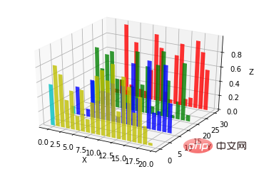

九、子图绘制（subplot）

A-不同的2-D图形，分布在3-D空间，其实就是投影空间不空，对应code:

from mpl_toolkits.mplot3d import Axes3D
import numpy as np
import matplotlib.pyplot as plt
 
fig = plt.figure()
ax = fig.gca(projection='3d')
 
# Plot a sin curve using the x and y axes.
x = np.linspace(0, 1, 100)
y = np.sin(x * 2 * np.pi) / 2 + 0.5
ax.plot(x, y, zs=0, zdir='z', label='curve in (x,y)')
 
# Plot scatterplot data (20 2D points per colour) on the x and z axes.
colors = ('r', 'g', 'b', 'k')
x = np.random.sample(20*len(colors))
y = np.random.sample(20*len(colors))
c_list = []
for c in colors:
    c_list.append([c]*20)
# By using zdir='y', the y value of these points is fixed to the zs value 0
# and the (x,y) points are plotted on the x and z axes.
ax.scatter(x, y, zs=0, zdir='y', c=c_list, label='points in (x,z)')
 
# Make legend, set axes limits and labels
ax.legend()
ax.set_xlim(0, 1)
ax.set_ylim(0, 1)
ax.set_zlim(0, 1)
ax.set_xlabel('X')
ax.set_ylabel('Y')
ax.set_zlabel('Z')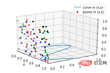

B-子图Subplot用法

与MATLAB不同的是，如果一个四子图效果，如：

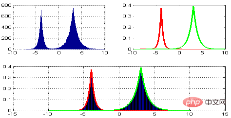
MATLAB：

subplot(2,2,1)
subplot(2,2,2)
subplot(2,2,[3,4])

Python:

subplot(2,2,1)
subplot(2,2,2)
subplot(2,1,2)

code:

import matplotlib.pyplot as plt
from mpl_toolkits.mplot3d.axes3d import Axes3D, get_test_data
from matplotlib import cm
import numpy as np
 
 
# set up a figure twice as wide as it is tall
fig = plt.figure(figsize=plt.figaspect(0.5))
 
#===============
#  First subplot
#===============
# set up the axes for the first plot
ax = fig.add_subplot(2, 2, 1, projection='3d')
 
# plot a 3D surface like in the example mplot3d/surface3d_demo
X = np.arange(-5, 5, 0.25)
Y = np.arange(-5, 5, 0.25)
X, Y = np.meshgrid(X, Y)
R = np.sqrt(X**2 + Y**2)
Z = np.sin(R)
surf = ax.plot_surface(X, Y, Z, rstride=1, cstride=1, cmap=cm.coolwarm,
                       linewidth=0, antialiased=False)
ax.set_zlim(-1.01, 1.01)
fig.colorbar(surf, shrink=0.5, aspect=10)
 
#===============
# Second subplot
#===============
# set up the axes for the second plot
ax = fig.add_subplot(2,1,2, projection='3d')
 
# plot a 3D wireframe like in the example mplot3d/wire3d_demo
X, Y, Z = get_test_data(0.05)
ax.plot_wireframe(X, Y, Z, rstride=10, cstride=10)
 
plt.show()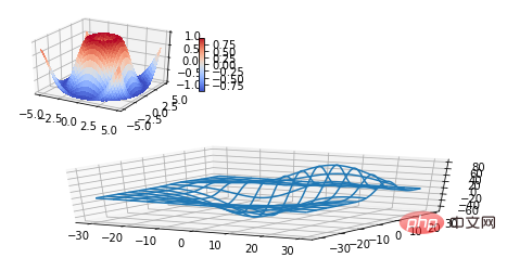

补充：

文本注释的基本用法：

code:

from mpl_toolkits.mplot3d import Axes3D
import matplotlib.pyplot as plt
 
 
fig = plt.figure()
ax = fig.gca(projection='3d')
 
# Demo 1: zdir
zdirs = (None, 'x', 'y', 'z', (1, 1, 0), (1, 1, 1))
xs = (1, 4, 4, 9, 4, 1)
ys = (2, 5, 8, 10, 1, 2)
zs = (10, 3, 8, 9, 1, 8)
 
for zdir, x, y, z in zip(zdirs, xs, ys, zs):
    label = '(%d, %d, %d), dir=%s' % (x, y, z, zdir)
    ax.text(x, y, z, label, zdir)
 
# Demo 2: color
ax.text(9, 0, 0, "red", color='red')
 
# Demo 3: text2D
# Placement 0, 0 would be the bottom left, 1, 1 would be the top right.
ax.text2D(0.05, 0.95, "2D Text", transform=ax.transAxes)
 
# Tweaking display region and labels
ax.set_xlim(0, 10)
ax.set_ylim(0, 10)
ax.set_zlim(0, 10)
ax.set_xlabel('X axis')
ax.set_ylabel('Y axis')
ax.set_zlabel('Z axis')
 
plt.show()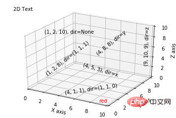

【相关推荐：Python3视频教程 】

以上是python绘制三维图的详细教程的详细内容。更多信息请关注PHP中文网其他相关文章！