这篇文章主要介绍了python数字图像处理之高级形态学处理,现在分享给大家,也给大家做个参考。一起过来看看吧
形态学处理,除了最基本的膨胀、腐蚀、开/闭运算、黑/白帽处理外,还有一些更高级的运用,如凸包,连通区域标记,删除小块区域等。
1、凸包
凸包是指一个凸多边形,这个凸多边形将图片中所有的白色像素点都包含在内。
函数为:
立即学习“Python免费学习笔记(深入)”;
1 | skimage.morphology.convex_hull_image(image)
|
登录后复制
输入为二值图像,输出一个逻辑二值图像。在凸包内的点为True, 否则为False
例:
1 2 3 4 5 6 7 8 9 10 11 12 13 14 15 16 17 | import matplotlib.pyplot as plt
from skimage import data,color,morphology
img=color.rgb2gray(data.horse())
img=(img<0.5)*1
chull = morphology.convex_hull_image(img)
fig, axes = plt.subplots(1,2,figsize=(8,8))
ax0, ax1= axes.ravel()
ax0.imshow(img,plt.cm.gray)
ax0.set_title('original image')
ax1.imshow(chull,plt.cm.gray)
ax1.set_title('convex_hull image')
|
登录后复制
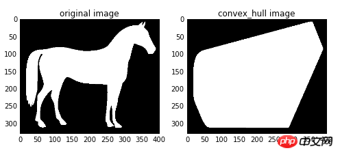
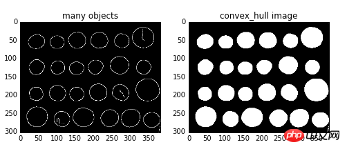
convex_hull_image()是将图片中的所有目标看作一个整体,因此计算出来只有一个最小凸多边形。如果图中有多个目标物体,每一个物体需要计算一个最小凸多边形,则需要使用convex_hull_object()函数。
函数格式:skimage.morphology.convex_hull_object(image,neighbors=8)
输入参数image是一个二值图像,neighbors表示是采用4连通还是8连通,默认为8连通。
例:
1 2 3 4 5 6 7 8 9 10 11 12 13 14 15 16 17 18 | import matplotlib.pyplot as plt
from skimage import data,color,morphology,feature
img=color.rgb2gray(data.coins())
edgs=feature.canny(img, sigma=3, low_threshold=10, high_threshold=50)
chull = morphology.convex_hull_object(edgs)
fig, axes = plt.subplots(1,2,figsize=(8,8))
ax0, ax1= axes.ravel()
ax0.imshow(edgs,plt.cm.gray)
ax0.set_title('many objects')
ax1.imshow(chull,plt.cm.gray)
ax1.set_title('convex_hull image')
plt.show()
|
登录后复制
2、连通区域标记
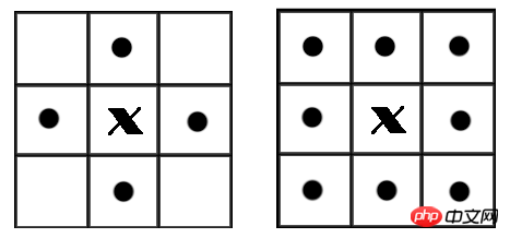
在二值图像中,如果两个像素点相邻且值相同(同为0或同为1),那么就认为这两个像素点在一个相互连通的区域内。而同一个连通区域的所有像素点,都用同一个数值来进行标记,这个过程就叫连通区域标记。在判断两个像素是否相邻时,我们通常采用4连通或8连通判断。在图像中,最小的单位是像素,每个像素周围有8个邻接像素,常见的邻接关系有2种:4邻接与8邻接。4邻接一共4个点,即上下左右,如下左图所示。8邻接的点一共有8个,包括了对角线位置的点,如下右图所示。
在skimage包中,我们采用measure子模块下的label()函数来实现连通区域标记。
函数格式:
1 | skimage.measure.label(image,connectivity=None)
|
登录后复制
参数中的image表示需要处理的二值图像,connectivity表示连接的模式,1代表4邻接,2代表8邻接。
输出一个标记数组(labels), 从0开始标记。
1 2 3 4 5 6 7 8 9 10 11 12 13 14 15 16 17 18 19 20 21 22 23 24 25 26 27 28 29 30 | import numpy as np
import scipy.ndimage as ndi
from skimage import measure,color
import matplotlib.pyplot as plt
def microstructure(l=256):
n = 5
x, y = np.ogrid[0:l, 0:l]
mask = np.zeros((l, l))
generator = np.random.RandomState(1)
points = l * generator.rand(2, n**2)
mask[(points[0]).astype(np.int), (points[1]).astype(np.int)] = 1
mask = ndi.gaussian_filter(mask, sigma=l/(4.*n))
return mask > mask.mean()
data = microstructure(l=128)*1
labels=measure.label(data,connectivity=2)
dst=color.label2rgb(labels)
print('regions number:',labels.max()+1)
fig, (ax1, ax2) = plt.subplots(1, 2, figsize=(8, 4))
ax1.imshow(data, plt.cm.gray, interpolation='nearest')
ax1.axis('off')
ax2.imshow(dst,interpolation='nearest')
ax2.axis('off')
fig.tight_layout()
plt.show()
|
登录后复制
在代码中,有些地方乘以1,则可以将bool数组快速地转换为int数组。
结果如图:有10个连通的区域,标记为0-9

如果想分别对每一个连通区域进行操作,比如计算面积、外接矩形、凸包面积等,则需要调用measure子模块的regionprops()函数。该函数格式为:
1 | skimage.measure.regionprops(label_image)
|
登录后复制
返回所有连通区块的属性列表,常用的属性列表如下表:
| 属性名称 |
类型 |
描述 |
| area |
int |
区域内像素点总数 |
| bbox |
tuple |
边界外接框(min_row, min_col, max_row, max_col) |
| centroid |
array |
质心坐标 |
| convex_area |
int |
凸包内像素点总数 |
| convex_image |
ndarray |
和边界外接框同大小的凸包 |
| coords |
ndarray |
区域内像素点坐标 |
| Eccentricity |
float |
离心率 |
| equivalent_diameter |
float |
和区域面积相同的圆的直径 |
| euler_number |
int |
区域欧拉数 |
| extent |
float |
区域面积和边界外接框面积的比率 |
| filled_area |
int |
区域和外接框之间填充的像素点总数 |
| perimeter |
float |
区域周长 |
| label |
int |
区域标记 |
3、删除小块区域
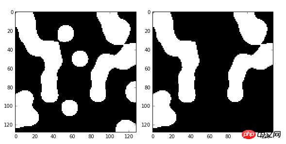
有些时候,我们只需要一些大块区域,那些零散的、小块的区域,我们就需要删除掉,则可以使用morphology子模块的remove_small_objects()函数。
函数格式:skimage.morphology.remove_small_objects(ar,min_size=64,connectivity=1,in_place=False)
参数:
ar: 待操作的bool型数组。
min_size: 最小连通区域尺寸,小于该尺寸的都将被删除。默认为64.
connectivity: 邻接模式,1表示4邻接,2表示8邻接
in_place: bool型值,如果为True,表示直接在输入图像中删除小块区域,否则进行复制后再删除。默认为False.
返回删除了小块区域的二值图像。
1 2 3 4 5 6 7 8 9 10 11 12 13 14 15 16 17 18 19 20 21 22 23 24 25 26 | import numpy as np
import scipy.ndimage as ndi
from skimage import morphology
import matplotlib.pyplot as plt
def microstructure(l=256):
n = 5
x, y = np.ogrid[0:l, 0:l]
mask = np.zeros((l, l))
generator = np.random.RandomState(1)
points = l * generator.rand(2, n**2)
mask[(points[0]).astype(np.int), (points[1]).astype(np.int)] = 1
mask = ndi.gaussian_filter(mask, sigma=l/(4.*n))
return mask > mask.mean()
data = microstructure(l=128)
dst=morphology.remove_small_objects(data,min_size=300,connectivity=1)
fig, (ax1, ax2) = plt.subplots(1, 2, figsize=(8, 4))
ax1.imshow(data, plt.cm.gray, interpolation='nearest')
ax2.imshow(dst,plt.cm.gray,interpolation='nearest')
fig.tight_layout()
plt.show()
|
登录后复制
在此例中,我们将面积小于300的小块区域删除(由1变为0),结果如下图:
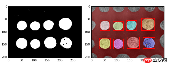
4、综合示例:阈值分割+闭运算+连通区域标记+删除小区块+分色显示
1 2 3 4 5 6 7 8 9 10 11 12 13 14 15 16 17 18 19 20 21 22 23 24 25 26 27 28 29 30 31 32 33 34 35 36 | import numpy as np
import matplotlib.pyplot as plt
import matplotlib.patches as mpatches
from skimage import data,filter,segmentation,measure,morphology,color
image = data.coins()[50:-50, 50:-50]
thresh =filter.threshold_otsu(image)
bw =morphology.closing(image > thresh, morphology.square(3))
cleared = bw.copy()
segmentation.clear_border(cleared)
label_image =measure.label(cleared)
borders = np.logical_xor(bw, cleared)
label_image[borders] = -1
image_label_overlay =color.label2rgb(label_image, image=image)
fig,(ax0,ax1)= plt.subplots(1,2, figsize=(8, 6))
ax0.imshow(cleared,plt.cm.gray)
ax1.imshow(image_label_overlay)
for region in measure.regionprops(label_image):
if region.area < 100:
continue
minr, minc, maxr, maxc = region.bbox
rect = mpatches.Rectangle((minc, minr), maxc - minc, maxr - minr,
fill=False, edgecolor='red', linewidth=2)
ax1.add_patch(rect)
fig.tight_layout()
plt.show()
|
登录后复制
以上就是python数字图像处理之高级形态学处理的详细内容,更多请关注php中文网其它相关文章!


 广告
广告
![ThinkPHP5快速开发企业站点[全程实录]](https://img.php.cn/upload/course/000/000/068/6253d918a3ce7278.png)


 788
788